Understanding Latent Dirichlet Allocation (4) Gibbs Sampling
In the last article, I explained LDA parameter inference using variational EM algorithm and implemented it from scratch. In this post, let’s take a look at another algorithm proposed in the original paper that introduced LDA to derive approximate posterior distribution: Gibbs sampling. In addition, I would like to introduce and implement from scratch a collapsed Gibbs sampling method that can efficiently fit topic model to the data.
This article is the fourth part of the series “Understanding Latent Dirichlet Allocation”.
- Problem setting in the original paper
- “Model with admixture”
- Gibbs sampling
- Collapsed Gibbs sampling
- Python implementation from scratch
Problem setting in the original paper
Pritchard and Stephens (2000) originally proposed the idea of solving population genetics problem with three-level hierarchical model. The problem they wanted to address was “inference of population struture using multilocus genotype data.” For those who are not familiar with population genetics, this is basically a clustering problem that aims to cluster individuals into clusters (population) based on similarity of genes (genotype) of multiple prespecified locations in DNA (multilocus).
The researchers proposed two models: one that only assigns one population to each individuals (“model without admixture”), and another that assigns mixture of populations (“model with admixture”). The latter is the model that later termed as LDA. Before we get to the inference step, I would like to briefly cover the original model with the terms in population genetics, but with notations I used in the previous articles.
“Model with admixture”
In population genetics setup, our notations are as follows:
- $V$ is the total number of possible alleles in every loci.
- $w_n$: genotype of the $n$-th locus. One-hot encoded so that $w_n^i=1$ and $w_n^j=0, \forall j\ne i$ for one $i\in V$.
- $z_n$: population of origin of $w_n$.
- $\mathbf{w}_d=(w_{d1},\cdots,w_{dN})$: genotype of $d$-th individual at $N$ loci.
- $D = (\mathbf{w}_1,\cdots,\mathbf{w}_M)$: whole genotype data with $M$ individuals.
Generative process of genotype of $d$-th individual $\mathbf{w}_{d}$ with $k$ predefined populations described on the paper is a little different than that of Blei et al. (2003).
- $\beta_k \sim \mathcal{D}_V(\eta)$.
- $\theta_d \sim \mathcal{D}_k(\alpha)$. $\theta_{di}$ is the probability that $d$-th individual’s genome is originated from population $i$.
- for $n=1,\cdots,N$:
- $z_{dn}$ is chosen with probability $P(z_{dn}^i=1|\theta_d,\beta)=\theta_{di}$.
- $w_{dn}$ is chosen with probability $P(w_{dn}^i=1|z_{dn},\theta_d,\beta)=\beta_{ij}$.
Since $\beta$ is independent to $\theta_d$ and affects the choice of $w_{dn}$ only through $z_{dn}$, I think it is okay to write $P(z_{dn}^i=1|\theta_d)=\theta_{di}$ instead of formula at 2.1 and $P(w_{dn}^i=1|z_{dn},\beta)=\beta_{ij}$ instead of 2.2.
The only difference between this and (vanilla) LDA that I covered so far is that $\beta$ is considered a Dirichlet random variable here. In fact, this is exactly the same as smoothed LDA described in Blei et al. (2003) which will be described in the next article.
Gibbs sampling
To estimate the intracktable posterior distribution, Pritchard and Stephens (2000) suggested using Gibbs sampling. Gibbs sampling is a method of Markov chain Monte Carlo (MCMC) that approximates intractable joint distribution by consecutively sampling from conditional distributions. Suppose we want to sample from joint distribution $p(x_1,\cdots,x_n)$. Assume that even if directly sampling from it is impossible, sampling from conditional distributions $p(x_i|x_1\cdots,x_{i-1},x_{i+1},\cdots,x_n)$ is possible. Then repeatedly sampling from conditional distributions as follows
- Repeat:
- Sample $x_1^{(t+1)}$ from $p(x_1|x_2^{(t)},\cdots,x_n^{(t)})$.
- Sample $x_2^{(t+1)}$ from $p(x_2|x_1^{(t+1)}, x_3^{(t)},\cdots,x_n^{(t)})$.
- $~~\vdots$
- Sample $x_n^{(t+1)}$ from $p(x_n|x_1^{(t+1)},\cdots,x_{n-1}^{(t+1)})$.
gives us an approximate sample $(x_1^{(m)},\cdots,x_n^{(m)})$ that can be considered as sampled from the joint distribution for large enough $m$’s.
Below is a paraphrase, in terms of familiar notation, of the detail of the Gibbs sampler that samples from posterior of LDA. Let
\[\mathbf{n}_i = (n_{i1},\cdots,n_{iV}) \\ \mathbf{m}_d = (m_{d1},\cdots,m_{dk})\]where $n_{ij}$ the number of occurrence of word $j$ under topic $i$, $m_{di}$ is the number of loci in $d$-th individual that originated from population $i$.
-
Update $\beta^{(t+1)}$ with a sample from $\beta_i|\mathbf{w},\mathbf{z}^{(t)} \sim \mathcal{D}_V(\eta+\mathbf{n}_i)$.
-
Update $\theta^{(t+1)}$ with a sample from $\theta_d|\mathbf{w},\mathbf{z}^{(t)} \sim \mathcal{D}_k(\alpha^{(t)}+\mathbf{m}_d)$.
-
Update $\mathbf{z}_d^{(t+1)}$ with a sample by probability
\[P(z_{dn}^i=1|\mathbf{w},\beta^{(t+1)}) = \frac{\theta_{di}\beta_{iw_{dn}}^{(t+1)}}{\sum_{d=1}^M \theta_{di}\beta_{iw_{dn}}^{(t+1)}}.\] -
Update $\alpha^{(t+1)}$ by the following process:
- Sample $\alpha’$ from $\mathcal{N}(\alpha^{(t)}, \sigma_{\alpha^{(t)}}^{2})$ for some $\sigma_{\alpha^{(t)}}^2$.
- Let $a = \frac{p(\alpha’|\theta^{(t)},\mathbf{w},\mathbf{z}^{(t)})}{p(\alpha^{(t)}|\theta^{(t)},\mathbf{w},\mathbf{z}^{(t)})} \cdot \frac{\phi_{\alpha’}(\alpha^{(t)})}{\phi_{\alpha^{(t)}}(\alpha’)}$.
- Do not update $\alpha^{(t+1)}$ if $\alpha’\le0$. Update $\alpha^{(t+1)}=\alpha’$ if $a \ge 1$, otherwise update it to $\alpha’$ with probability $a$.
The update rule in step 4 is called Metropolis-Hastings algorithm.
Collapsed Gibbs sampling
While the proposed sampler works, in topic modelling we only need to estimate document-topic distribution $\theta$ and topic-word distribution $\beta$. Griffiths and Steyvers (2002) boiled the process down to evaluating the posterior $P(\mathbf{z}|\mathbf{w}) \propto P(\mathbf{w}|\mathbf{z})P(\mathbf{z})$ which was intractable. Notice that we marginalized the target posterior over $\beta$ and $\theta$. This makes it a collapsed Gibbs sampler; the posterior is collapsed with respect to $\beta,\theta$.
Marginalizing the Dirichlet-multinomial distribution $P(\mathbf{w}, \beta | \mathbf{z})$ over $\beta$ from smoothed LDA, we get the posterior topic-word assignment probability
\[P(\mathbf{w}|\mathbf{z}) = \left( \frac{\Gamma(V\eta)}{\Gamma(\eta)^V} \right)^k \prod_{i=1}^k\frac{\prod_{j=1}^V \Gamma(n_{ij}+\eta)}{\Gamma(n_{i\cdot}+V\eta)}\]where $n_{ij}$ is the number of times word $j$ has been assigned to topic $i$, just as in the vanilla Gibbs sampler. Marginalizing another Dirichlet-multinomial $P(\mathbf{z},\theta)$ over $\theta$ yields
\[P(\mathbf{z}) = \left( \frac{\Gamma(k\alpha)}{\Gamma(\alpha)^k} \right)^M \prod_{d=1}^M \frac{\prod_{i=1}^k \Gamma(n_{di}+\alpha)}{\Gamma(n_{d\cdot}+k\alpha)}\]where $n_{di}$ is the number of times a word from document $d$ has been assigned to topic $i$. Multiplying these two equations, we get
\[P(z_{dn}^i=1 | \mathbf{z}_{(-dn)},\mathbf{w}) \propto \frac{n_{(-dn),iw_{dn}}+\eta}{n_{(-dn),i\cdot}+V\eta} \frac{n_{(-dn),di}+\alpha}{n_{(-dn),d\cdot}+k\alpha},\]where $\mathbf{z}_{(-dn)}$ is the word-topic assignment for all but $n$-th word in $d$-th document, $n_{(-dn)}$ is the count that does not include current assignment of $z_{dn}$.
The first term can be viewed as a (posterior) probability of $w_{dn}|z_i$ (i.e. $\beta_{dni}$), and the second can be viewed as a probability of $z_i$ given document $d$ (i.e. $\theta_{di}$). We run sampling by sequentially sample $z_{dn}^{(t+1)}$ given $\mathbf{z}_{(-dn)}^{(t)}, \mathbf{w}$ after one another.
After sampling $\mathbf{z}|\mathbf{w}$ with Gibbs sampling, we recover $\theta$ and $\beta$ with
\[\hat\beta_{iw_n} = \frac{n_{iw_n}+\eta}{n_{i\cdot}+V\eta}, \\ \hat\theta_{di} = \frac{n_{di}+\alpha}{n_{d\cdot}+k\alpha},\]which are marginalized versions of the first and second term of the last equation, respectively.
Python implementation from scratch
Here, I would like to implement the collapsed Gibbs sampler only, which is more memory-efficient and easy to code.
The sampler
This is the entire process of gibbs sampling, with some abstraction for readability.
def run_gibbs(docs, vocab, n_topic, n_gibbs=2000, verbose=True):
    """
    Run collapsed Gibbs sampling
    """
    # initialize required variables
    _init_gibbs(docs, vocab, n_topic, n_gibbs)

    if verbose:
        print("\n", "="*10, "START SAMPLER", "="*10)

    # run the sampler
    for t in range(n_gibbs):
        for d in range(M):
            for n in range(N[d]):
                w_dn = docs[d][n]

                # decrement counter
                i_t = assign[d, n, t]  # previous assignment
                n_iw[i_t, w_dn] -= 1
                n_di[d, i_t] -= 1

                # assign new topics
                prob = _conditional_prob(w_dn, d)
                i_tp1 = np.argmax(np.random.multinomial(1, prob))

                # increment counter with new assignment
                n_iw[i_tp1, w_dn] += 1
                n_di[d, i_tp1] += 1
                assign[d, n, t+1] = i_tp1

        # print out status
        if verbose & ((t+1) % 50 == 0):
            print(f"Sampled {t+1}/{n_gibbs}")
In _init_gibbs(), instantiate variables (numbers V, M, N, k and hyperparameters alpha, eta and counters and assignment table n_iw, n_di, assign).
def _init_gibbs(docs, vocab, n_topic, n_gibbs=2000):
    """
    Initialize t=0 state for Gibbs sampling.
    Replace initial word-topic assignment
    ndarray (M, N, N_GIBBS) in-place.
    """
    # initialize variables
    init_lda(docs, vocab, n_topic=n_topic, gibbs=True)

    # word-topic assignment
    global assign
    N_max = max(N)
    assign = np.zeros((M, N_max, n_gibbs+1), dtype=int)
    print(f"assign: dim {assign.shape}")

    # initial assignment
    for d in range(M):
        for n in range(N[d]):
            # randomly assign topic to word w_{dn}
            w_dn = docs[d][n]
            assign[d, n, 0] = np.random.randint(k)

            # increment counters
            i = assign[d, n, 0]
            n_iw[i, w_dn] += 1
            n_di[d, i] += 1
_conditional_prob() is the function that calculates $P(z_{dn}^i=1 | \mathbf{z}_{(-dn)},\mathbf{w})$ using the multiplicative equation above.
def _conditional_prob(w_dn, d):
    """
    P(z_{dn}^i=1 | z_{(-dn)}, w)
    """
    prob = np.empty(k)

    for i in range(k):
        # P(w_dn | z_i)
        _1 = (n_iw[i, w_dn] + eta) / (n_iw[i, :].sum() + V*eta)
        # P(z_i | d)
        _2 = (n_di[d, i] + alpha) / (n_di[d, :].sum() + k*alpha)

        prob[i] = _1 * _2

    return prob / prob.sum()
After running run_gibbs() with appropriately large n_gibbs, we get the counter variables n_iw, n_di from posterior, along with the assignment history assign where [:, :, t] values of it are word-topic assignment at sampling $t$-th iteration.
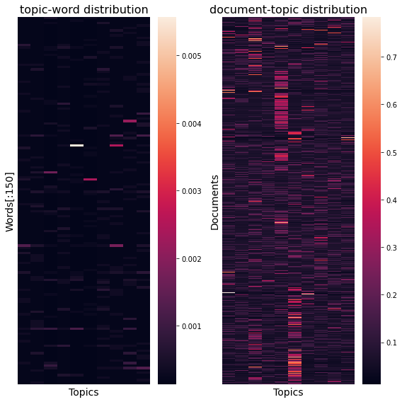
Recover $\hat\beta$ and $\hat\theta$
Now we need to recover topic-word and document-topic distribution from the sample.
β̂ = np.empty((k, V))
θ̂ = np.empty((M, k))

for j in range(V):
    for i in range(k):
        β̂[i, j] = (n_iw[i, j] + eta) / (n_iw[i, :].sum() + V*eta)

for d in range(M):
    for i in range(k):
        θ̂[d, i] = (n_di[d, i] + alpha) / (n_di[d, :].sum() + k*alpha)
Finally we can plot it as a heatmap.
Full code and result are available here (GitHub).
References
- Pritchard, Stephens, Donnelly. 2000. Inference of Population Structure Using Multilocus Genotype Data. Genetics. 155: 945–959.
- Griffiths, Steyvers. 2004. Finding scientific topics. Proceedings of the National Academy of Sciences of the United States of America. 101: 5228-5235.