1. Brief Introduction to Nonparametric function estimation
The [Nonparametric] series of posts is my memo on the lecture Nonparametric Function Estimation (Spring, 2021) by Prof. Byeong U. Park. The lecture is mainly focused on kernel smoothing, while also briefly covers other nonparametric methods such as MARS.
Nonparametric model
Assume the data $(\mathbf{X}_i, Y_i)$ are random, where $Y_i \in \mathbb{R}$ and $\mathbf{X}_i \in [0,1]^d$. Our main goal is to estimate the model $f$ that best describes the relationship between $\mathbf{X}$ and $Y$, using the observations $(Y_i, \mathbf{X}_i)_{i=1}^n$.
\[Y_i = f(\mathbf{X}_i) + \epsilon_i,~ 1\le i\le n.\]In nonparametric estimation, $f$ is not, or nearly specified. This makes dimension of parameter space infinite, which is called “nonparametric”. In order to identify such $f$, conditional expectation of unobserved intrinsic error $\epsilon_i$’s’ should be zero: $E(\epsilon\vert\mathbf{X}_i)=0$.
Note that the problem we set is an ill-posed problem: the dimension of parameter space is $\infty$ while the sample size is finite $n$. Several solutions have been proposed.
- Method of sieves. As the name speaks for itself, this method approximate the true model by setting a sequence of finite dimensional models $(\hat f_n)$ such that as $n\to\infty,$ the dimension of $\hat f_n$ also grows to infinity. A sequence of polynomials, spline (piecewise fitted polynomials) and wavelet is some examples of it.
- Kernel smoothing. Using the kernel function, use weighted local mean to approximate the true model. Locally constant / linear / $\cdots$ regression are included.
Polynomial approximation
It pretty much is one of the simpliest method: we approximate $f$ with a sequence of polynomials $\hat f_n$ of order $n$. In theory, as $n$ grows to infinity, $\hat f_n$ can well approximate $f$. However when fitted to real data, it usually requires very large $n$ to approximate well. This might lead to overly complex model (overfitting).
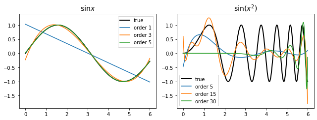
As we can see, polynomial fitting does not produce useful result when the true function behaves differently in different regions of its domain.
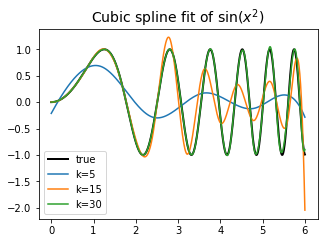
Splines
The problem of polynomial fitting is that it fails to address local context. To capture local behavior of the model, splines split the domain with preselected $K$ points
\[\tau_1 < \tau_2 < \cdots < \tau_K\]which is called knots. In each of the $(K+1)$ disjoint regions, we fit $(K+1)$ different polynomials of order $\ell$. Resulting function is the spline function of order $\ell$. To smoothly connect polynomials with each other, we constrain them to have $(\ell-1)$th continuous derivative at the knots.
To fit a spline of order $\ell$ with $K$ knots, we need
\[\underbrace{(K+1)(\ell+1)}_{\substack{\text{$\ell$ polynomials in} \\ \text{$(K+1)$ regions}}} - \underbrace{K\cdot\ell}_\text{constraint} = K + \ell + 1\]parameters. In fact, spline functions can be represented as
\[f(x) = \beta_0 + \beta_1 x + \cdots + \beta_\ell x^\ell + \sum_{j=1}^K \beta_{\ell + j} (x-\tau_j)^\ell_+. \tag{1}\]As $K \to \infty,$ the dimension of parameter space grows to infinity. $\ell$ is usually fixed to $\sim 3.$
While splines gives meaningful results, the process of fitting the model is similar to that of parametric model ((1) is merely a multiple linear regression). Hence this lecture focuses on kernel smoothing method which will be described below.
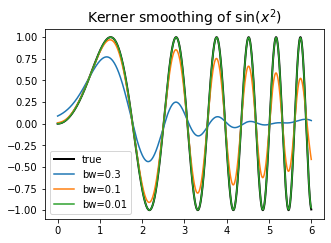
Kernel smoothing
Kernel smoothing can be viewed as a method to approximate the model by averaging the response with covariate values inside the interval $[x-h, x+h].$ $h$ is called bandwidth, or window width and it determines the size of local context to consider in approximation.
Using just simple local average, we get the locally constant regression function $\hat f$ as follows. This process of locally averaging the response is called smoothing since it “smooths out” the outlying responses.
\[\begin{aligned} \hat f(x) &:= \argmin_\alpha \int_{x-h}^{x+h} \left(f(u) - \alpha\right)^2 du \\ &= \frac{1}{2h} \int_{-1}^{1} \frac{u-x}{h} f(u) du. \end{aligned} \tag{2}\]More generally, we can use weighted local average of $f,$ using the value of kernel function $K$ as weights. $K$ is usually set so that responses associated with the inputs nearer to $x$ gets greater weights.
\[\begin{aligned} \hat f(x) &:= \argmin_\alpha \int \left(f(u) - \alpha\right)^2 K\left(\frac{u-x}{h}\right) du \\ &= \left( \int K\left(\frac{u-x}{h}\right) du \right)^{-1} \int K\left(\frac{u-x}{h}\right) f(u) du. \end{aligned} \tag{3}\]The interval of integration is defined in terms of the support of the kernel function $\text{supp.} K$. For instance, if $K(x) = \mathbf{1}_{[-1, 1]}(x),$ then (3) becomes the same as (2).
Appendix
References
- Nonparametric Function Estimation (Spring, 2021) @ Seoul National University, Republic of Korea (instructor: Prof. Byeong U. Park).