Understanding Skip Gram
Skip gram is one of the most utilized word embedding model to date. It was introduced at the same time with continuous bag-of-words (CBoW) together named as Word2Vec by Google researchers.
Skip gram is based on the distributional hypothesis where words with similar distribution is considered to have similar meanings. Recall that even though the NLPM was simple, it had myriads of parameters to be optimized. Researchers of skip gram suggested a model with less parameters along with the novel methods to make optimization step more efficient.
Vanilla skip gram
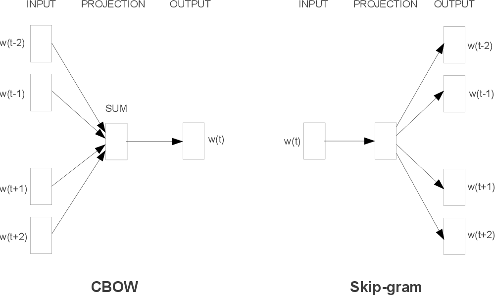
Main idea is to optimize model so that if it is queried with a word, it should correctly guess all the context ($\pm$2 in the figure) words. That is,
\[y = \text{softmax}(Ux)\]where $x,y$ are one-hot encoded word vector, $U$ is the embedding matrix. With the same dataset, training set for skip gram can be much larger than that of NPLM since it can have $2c$ samples ($w_t:w_{t-c}$, $\cdots$, $w_t:w_{t-1}$, $w_t:w_{t+1}$, $\cdots$, $w_t:w_{t+c}$) while NPLM and other n-gram based models have one ($(w_{t-c}, \cdots w_{t-1}, w_{t+1}, \cdots, w_{t+c}):w_t$). In addition, $U$ is the only parameters to be optimized, which has $|V|\times D$ values in it where $|V|$ is the size of the vocabulary, $D$ is the embedding dimension.
Subsampling
To make optimization more efficient, the researchers subsampled the dataset so that words with high occurence can be ignored while training. To be specific, they calculated the subsampling probability to be
\[P(w_i) = \left( \sqrt{\frac{z(w_i)}{t}} + 1 \right) \times \frac{t}{z(w_i)}\]where $t$ is a hyperparameter that suggested to be 1e-3, $z(w_i)$ is the fraction of occurence of word $w_i$. We include $w_i$ to the training set with probability $P(w_i)$.
import random
import math

def subsample_prob(word, t=1e-3):
    z = freq[word_to_ix[word]] / sum_freq
    return (math.sqrt(z/t) + 1) * t/z

words_subsample = [w for w in words if random.random() < subsample_prob(w)]
Negative sampling
The vanilla model has a softmax function as its final activation. The problem is it is computationally expensive since it has to output $|V|$-dimensional vector. To avoid calculating high-dimensional softmax, the researchers proposed negative sampling.
Instead of training the model to output one word out of $|V|$ vocabulary when a word is feeded, we feed the model with a pair of two words and then train it to predict if it is the right pair (positive sample) or not (negative sample). The ratio between positive and negative samples is $1:2\sim5$ for large text and $1:5\sim20$ for small text.
When generating negative samples, it is better to use words with less frequency more often than its actual frequency. To be specific, we adjust the negative sampling probability to be
\[P(w_i) = \frac{f(w_i)^{3/4}}{\sum f(w_i)^{3/4}}\]where $f(w_i)$ is the frequency of $i$th word.
def build_sample(words, vocab=vocab, freq=freq, c=2, k=2, use_neg_prob=True):
    """
    build dataset with negative sampling. Default context size is `c=2`.
    Ratio between positive and negative samples will be 1:k (default: `k=2`).
    """
    x, y = [], []
    vocab = np.array(vocab)
    freq = np.array(freq)
    wordix = seq_to_ix(words)
    for i in tqdm(range(len(words)-c)):
        current = wordix[i]
        context_pos = wordix[i+1:i+c+1]

        # negative sampling probability
        pos_idx_adj = np.sort(np.unique(wordix[i:i+c+1]))
        pos_idx_adj -= np.arange(len(pos_idx_adj))
        neg_idx = np.arange(len(freq)-c-1)
        neg_idx += np.searchsorted(pos_idx_adj, neg_idx, side='right')
        freq_neg = freq[neg_idx]

        if use_neg_prob:
            probs = reweight_prob(freq_neg)
        else:
            probs = freq_neg / freq_neg.sum()

        context_neg = seq_to_ix(np.random.choice(vocab[neg_idx],
                                                 c*k,
                                                 replace=False,
                                                 p=probs))

        # positive samples + negative samples
        #context = context_pos + context_neg
        #current = [current] * len(context)
        labels = [[1] + [0] * k] * c

        for j, x_pos in enumerate(context_pos):
            x.append([(current, x_pos)] + list(zip([current]*c, context_neg[j:j+c])))
        y += labels

    return x, y
With negative sampling, out model becomes a binary classification model
\[x = \{(t_+, c_+), (t_{-,j}, c_{-,j}): j=1, \cdots, k\}, \\ u_i = Ut_i, \\ v_i = Vc_i,\\ \hat y_i = \sigma\left( u_i'v_i \right) = \frac{1}{1 + e^{-u_i'v_i}}\]where $t_{ij}$ is the one-hot encoded target word vector, $v_{ij}$ is the context word vector, $U,V$ are embeddings, $y_{ij}\in{0, 1}$ is the target label.
Our goal is to maximize the cross entropy loss
\[\text{CE}(y, \hat y) = - \sum_{i=+,-} \sum_{j=1}^k y_{ij} \log \hat y_{ij} + (1-y_{ij}) \log (1-\hat y_{ij}).\]PyTorch implementation
class SkipGram(nn.Module):
    def __init__(self, vocab_size, embedding_dim):
        super(SkipGram, self).__init__()

        # embeddings
        self.embedding_u = nn.Embedding(vocab_size, embedding_dim)
        self.embedding_v = nn.Embedding(vocab_size, embedding_dim)

    def forward(self, x):
        # input should be of shape [batch_size, 1+k, 2]
        # split positive and negative sample
        batch_size = x.shape[0]
        x_pos_1, x_pos_2 = x[:, 0, :].T
        x_neg_1, x_neg_2 = x[:, 1:, :].T

        # log-likelihood w.r.t. x_pos
        u = self.embedding_u(x_pos_1)
        v = self.embedding_v(x_pos_2)
        x_pos = (u * v).sum(dim=1).view(1, -1)

        # log-likelihood w.r.t. x_neg
        u = self.embedding_u(x_neg_1)
        v = self.embedding_v(x_neg_2)
        x_neg = (u * v).sum(dim=2)

        x = torch.cat((x_pos, x_neg)).T

        return x

model = SkipGram(VOCAB_SIZE, EMBEDDING_DIM)
Use BCEWithLogitsLoss as loss function.
optimizer = optim.SGD(model.parameters(), lr=0.05, momentum=0.9)
criterion = nn.BCEWithLogitsLoss()
Full result can be seen here (GitHub repo).
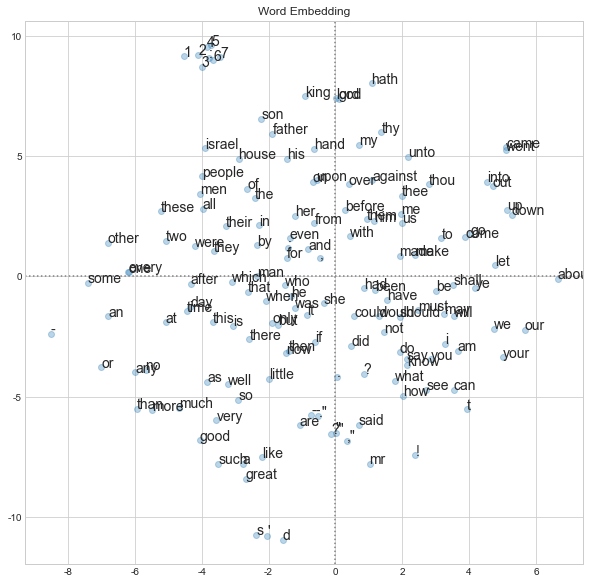
Embedding quality
Use t-SNE to reduce the dimension of embedding to 2, and plot each word vectors. The 150 most frequent words are plotted.
Top 5 most similar words result seems good as well.
QUERY   RESULT
angel : ['isaiah', 'spake', 'jesus', 'lord', 'rachel']
snow  : ['mid', 'ice', 'storm', 'bodily', 'wind']
love  : ['sing', 'esteem', 'faith', 'tempt', 'rejoice']
death : ['life', 'hell', 'presence', 'battle', 'dead']
References
- Mikolov et al. 2013. Efficient Estimation of Word Representations in Vector Space. International Conference on Learning Representations.
- Mikolov et al. 2013. Distributed Representations of Words and Phrases and their Compositionality. Advances in Neural Information Processing Systems, 26.
- Lee. 2019. 한국어 임베딩 (Embedding Korean). 에이콘 출판사.