Understanding FastText
While previous word embedding models focused on word-level features such as n-gram, FastText additionally focused on character-level features (subwords) to add flexibility to the model.
Subwords
Suppose that a word where was not in the training set. Previous to FastText, if where appears on the test set, then embedding models ignore unseen words and only use words in training set to embed sentences. This might seem reasonable, but we are missing quite information while doing so.
The key idea behind FastText is that subwords, character-level n-gram of each word, can be used to train word representation. The rationale is that similarly shaped words is more likely to have similar meanings (morphology). For example, where, who, when and why all have the 2-gram subword wh in common. This similarity in character composition has information that these words have similar semantics: the interogative.
Researchers carefully split words into subwords by adding special boundary symbols <, > which symbolize start of frame (sof) and end of frame (eof) respectively. Boundary symbols help the model to identify difference between similar but semantically different subwords. For instance, <where> and <her> both have her as their 3-gram subword. However nearby subwords of <her> (<he, er>) is quite different than those of <where> (whe, ere).
FastText
Aside from the fact that it uses subword vectors to characterize word vectors, it is more or less the same as skip gram. It uses subsampling, negative sampling just like skip gram, and it is also a binary classification model.
\[s_{i,g} \in \mathcal{G}_{t_i}, \\ z_{i,g} = Zs_{i,g}, \\ u_i = \sum_{g\in\mathcal{G}_{t_i}} z_{i,g},~ v_i = Vc_i, \\ \hat y_i = \sigma\left( u_i'v_i \right) = \frac{1}{1 + e^{-u_i'v_i}}\]where $s_{i,g}$’s are subwords of $i$th word $t_i$, $c_i$ is the context word, $Z$ is the subword embedding, $V$ is the word embedding, $y_i\in{0, 1}$ is the target label. Note that subword-level embedding was not used for context words.
Our goal is to maximize the cross entropy loss
\[\text{CE}(y, \hat y) = - \sum_{i=+,-} \sum_{j=1}^k y_{ij} \log \hat y_{ij} + (1-y_{ij}) \log (1-\hat y_{ij}).\]PyTorch implementation
class FastText(nn.Module):
    def __init__(self, subvocab_size, vocab_size, embedding_dim):
        super(FastText, self).__init__()

        # adjust Long according to device type
        self.Long = torch.LongTensor if (device.type == "cpu") else torch.cuda.LongTensor

        # embeddings
        self.embedding_z = nn.EmbeddingBag(subvocab_size+1, embedding_dim, mode="sum") # +1 for empty
        self.embedding_z.weight.data[-1] = 0
        self.embedding_v = nn.Embedding(vocab_size, embedding_dim)

    def forward(self, x):
        # input should be of shape [batch_size, 1+k, 2]
        x_1, x_2 = x.T

        # get subwords
        k = x_1.shape[0]
        x_1_sub = self.Long([get_subword(x_1[i]) for i in range(k)])

        # log-likelihood: sum up subword vectors to get word vector
        u = torch.stack([self.embedding_z(subwords) for subwords in x_1_sub])
        v = self.embedding_v(x_2)
        y = (u * v).sum(dim=2).T

        return y
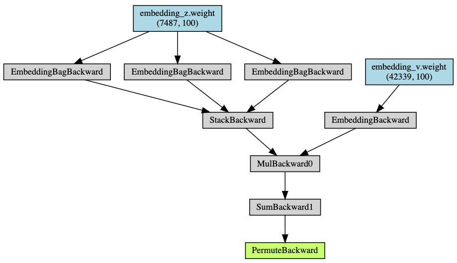
I used torch.nn.EmbeddingBag to speed up computing time. The computational graph looks like this:

Embedding quality
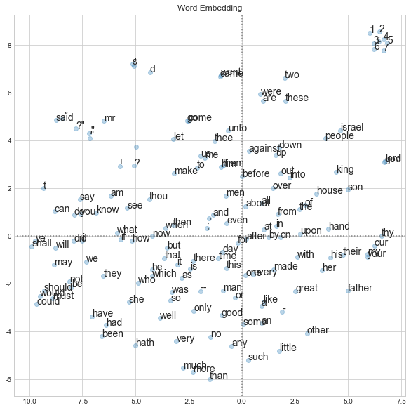
Use t-SNE to reduce the dimension of embedding to 2, and plot each word vectors. Only the 150 most frequent words are plotted.

Results are similar to that of skip gram, but FastText tends to embed words with similar morphology closer to each other (for example, (are, were) and (then, when)).
Top 5 most similar words result implies this property as well. Compare it to the result from skip gram.
QUERY   RESULTS
angel : ['angels', 'strangely', 'thus', 'saith', 'lord']
snow  : ['blue', 'figures', 'rolls', 'like', 'mud']
love  : ['loved', 'lovers', 'lover', 'my', 'thy']
death : ['thee', 'mercy', 'life', 'breath', 'judgment']
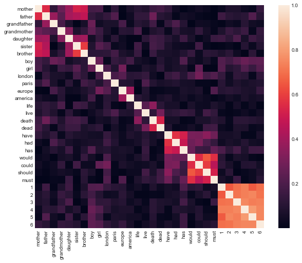
Cosine similarity heatmap agrees with the results.

Full results can be found here (notebook).
References
- Bojanowski et al. 2017. Enriching Word Vectors with Subword Information. Transactions of the Association for Computational Linguistics, 5, 135-146.
- Lee. 2019. 한국어 임베딩 (Embedding Korean). 에이콘 출판사.