Mutual information and Channel Capacity
From the definition of entropy, Shannon further defined information that the message $X$ and the recovered message $Y$ have in common. Using the the founding definitions from this and the previous article, we can develop a little more sophisticated theory.
Conditional entropy
Similar to how we defined the entropy, the conditional entropy of $X$ given $Y$ can be defined as
\[\begin{aligned} H(X\vert Y) &= -\sum_{x,y} p(x,y) \log p_{X|Y}(x|y) \\ &= -\sum_{x,y} p(x,y) \log \frac{p(x,y)}{p_Y(y)} \end{aligned}\]where $p_X$, $p_Y$ and $p$ are (joint) densities of $X$, $Y$ and $(X,Y),$ respectively. Note that
\[\begin{aligned} H(X\vert Y) &= -\sum_{x,y} p(x,y) \log \frac{p(x,y)}{p_Y(y)} \\ &= -\sum_{x,y} p(x,y) \log p(x,y) + \sum_{x,y} p(x,y) \log{p_Y(y)} \\ &= -\sum_{x,y} p(x,y) \log p(x,y) + \sum_{y} p(y) \log{p_Y(y)} \\ &= H(X,Y) - H(Y) \end{aligned} \tag{1}\label{1}\]Mutual information
Let $X$ and $Y$ be random variables, each with density $p_X$ and $p_Y$. The mutual information of $X$ and $Y$ is $$\begin{aligned} I(X;Y) &= H(X) - H(X|Y) \\ &= H(X) - H(Y|X) \\ &= H(X) + H(Y) - H(X,Y) \end{aligned}$$
The symmetricity of $I(\cdot;\cdot)$ is direct from the equation $\eqref{1}$.
Channel capacity
Definition
Let $X$ and $Y$ be random variables with density $p_X, p_Y,$ respectively. The channel density $C$ is defined as $$ C = \sup_{p_X(x)} I(X;Y) $$
Why is this quantity called the “capacity”? It turns out $C$ is the rate of transmission that can be sent reliably over the (noisy) channel between $X$ and $Y.$
Examples
(1) Consider a communication system of binary signal with noiseless channel. i.e.
\[\begin{cases} X=0 \implies Y=0 \text{ with prob. 1} \\ X=1 \implies Y=1 \text{ with prob. 1} \end{cases}\]In this setting, there is no uncertainty: $p_{X|Y}(x|y)=1$; we can fully decode the original signal. The channel capacity can be computed as follows.
\[I(X;Y) = H(X) - \cancel{H(X|Y)} = H(X) \\ \therefore C = \sup_{p_X(x)}H(X) = -\log_2(1/2) = 1.\]The second equality is achieved when $p_X(x)\equiv1/2.$ The result $C=1$ implies that one bit, which is in this case the entire information, can be reliably transmitted (per unit time1).
(2) This time, consider another binary signal transmitting system with noisy channel.
\[\begin{cases} X=0 \implies \begin{cases} Y=0 \text{ with prob. 0.5}\\ Y=1 \text{ with prob. 0.5}\\ \end{cases} \\ X=1 \implies \begin{cases} Y=0 \text{ with prob. 0.5}\\ Y=1 \text{ with prob. 0.5}\\ \end{cases} \end{cases}\]Then it is easy to show that $\mathbb P(Y=0)=\mathbb P(Y=1)=1/2$ and thus
\[\begin{aligned} I(X;Y) &= I(Y;X) \\ &= H(Y) - H(Y|X)\\ &= 1-1=0, \\ \end{aligned}\] \[\therefore C = \sup_{p_X(x)}0=0.\]which implies no information can be practically transferred.
Derivation of $C$
Random coding
For a message $M,$ let $x^{[n]}$ be a random (binary) code of length $n$ with each component be independent and identically distributed.
\[X^{[n]} = (X_1,\cdots,X_n), \\ X_i\in\{0,1\},~ X_i \overset{\text{i.i.d}}\sim p_X,~ 1\le i\le n\]Typical sequence
Suppose that $X_i \sim \text{Ber}(p).$ Consider the two realized sequences of length $n.$
\[(\underbrace{0,\cdots\cdots\cdots\cdots,0}_{(n(1-p)) \text{-many zeros}}, \underbrace{1,\cdots\cdots\cdot,1}_{(np) \text{-many ones}}) \tag{Seq 1}\label{Seq 1}\] \[(\underbrace{0,\cdots\cdots\cdots\cdots,0}_{n\text{-many zeros}}) \tag{Seq 2}\label{Seq 2}\]Notice that although the $\eqref{Seq 2}$ is more probable than the $\eqref{Seq 1}$ with probability $(1-p)^n$ if $p<0.5,$ as $n \to \infty$ an arbitrarily chosen sequence will be a permutation of $\eqref{Seq 1}$ with probability tending to one. Such sequence $x^{[n]}$ which is one of the limiting sequences in probability is called a $\varepsilon$-typical sequence of $X^{[n]}$. Typical sequence for cases other than binary code can also be defined similarly.
Note that for a $\varepsilon$-typical sequence $x^{[n]}$ of $X^{[n]}$ in any setting (not limited to the binary case), the log likelihood is given as
\[\begin{aligned} &\log_2 p(x^{[n]}) = \sum_{i=1}^n \log_2 p_X(x_i) \\ &= \log_2\left(\prod_{i=1}^n p_X(x_i)\right) \\ &= -n\sum_x p_X(x)\log_2p_X(x) \\ &= nH(X). \end{aligned}\]For a continuous density, instead of the exact value of log likelihood, we get the interval:
\[nH(X) - \varepsilon' \le \log_2 p(x^{[n]}) \le nH(X) + \varepsilon'\]where $\varepsilon’>0$ is a sufficiently small number.
The $\boldsymbol\varepsilon$-typical $\boldsymbol n$-tuple set (or simply “typical set”) is defined as a set of $\varepsilon$-typical sequences. To be specific, the $\varepsilon$-typical set $A_\varepsilon^n$ of $X^{[n]}$ is defined as
\[A_\varepsilon^n = \left\{ x^{[n]}:~ \frac1n\left|\sum_{i=1}^n \log_2 p_X(x_i)\right| \le H(X)+\varepsilon \right\}.\]One can intuitively get a glimpse of the following properties of a typical set. \(\begin{aligned} \text{(1) }&~ \mathbb P(X^{[n]} \in A_\varepsilon^n) \to 1 \text{ as } n\to\infty. \\ \text{(2) }&~ \mathbb P(x^{[n]}) = 2^{-nH(X)},~ \forall x^{[n]} \in A_\varepsilon^n. \\ \text{(3) }&~ |A_\varepsilon^n| = 2^{nH(X)}. \\ \end{aligned}\)
For two sequences $X^{[n]}$ and $Y^{[n]},$ where $Y^{[n]}$ is defined as before but with density $p_Y,$ we can also define the joint typical set in the same sense. For clarity, we denote $A_\varepsilon^n(X)$, $A_\varepsilon^n(Y)$ for the marginal one and $A_\varepsilon^n(X, Y)$ for the joint one. We say that $(x^{[n]}, y^{[n]})$ is jointly $\boldsymbol \varepsilon$-typical if $(x^{[n]}_ i, y^{[n]}_ i)$’s are i.i.d. and both $x^{[n]}$ and $y^{[n]}$ are $\varepsilon$-typical with respect to their marginal densities. Note that $x^{[n]} \in A_\varepsilon^n(X)$ and $y^{n} \in A_\varepsilon^n(Y)$ does not implies $(x^{[n]},y^{[n]}) \in A_\varepsilon^n(X,Y)$ but the converse holds by definition.
Decoding from a noisy channel
For sufficiently large $n\in\mathbb N,$ most of the realized sequences of $X^{[n]}$ and $Y^{[n]}$ are in the typical set $A_\varepsilon(X)$ and $A_\varepsilon^n(Y)$ respectively. It is also true that most of the realizations of $(X^{[n]}, Y^{[n]})$ are in $A_\varepsilon^n(X,Y).$
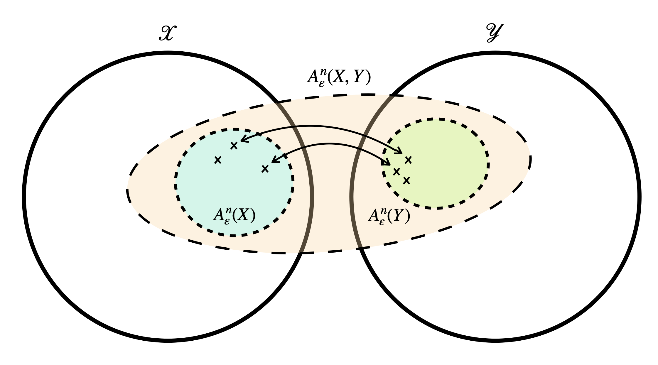
Figure 1. Decoding by typical sets
Using this fact, if we observe the transmitted signal $y^{[n]}$ then from the joint typical set we can, with probability tending to one, estimate the original signal $x^{[n]}.$
We can compute the total number of combinations of $\varepsilon$-typical sequences of $X^{[n]}$ and $Y^{[n]}$ is $2^{nH(X)}\cdot2^{nH(Y)}.$ Similarly, we can compute the total number of jointly $\varepsilon$-typical sequences to be $2^{nH(X,Y)}.$ From these, we get the cardinality of jointly $\varepsilon$-typical set:
\[\begin{aligned} &2^{nH(X)}\cdot2^{nH(Y)}/2^{nH(X,Y)} \\ &= 2^{n{(H(X) + H(Y) - H(X,Y))}} \\ &= 2^{nI(X;Y)}. \end{aligned}\tag{2}\label{2}\]In fact, it is the upper bound of the number of distinguishable messages. Since $I(X;Y)$ determines the rate of which the number of distinguishable messages increases as $n$ grows, we define the channel capacity as the value of $I(X,Y)$ in the best case scenario (the supremum with respect to $p_X$).
Rate distortion theory
Instead of a signal transmission setting, let’s now consider a signal compression setting. This time, we want to compress the signal as much as possible with the distortion of information under control. This can be written as follows.
First, define the distortion of information between the two sequences
\[d(x^{[n]}, z^{[n]}) = \frac1n \sum_{i=1}^n d(x_i, z_i)\]where $d(x_i, z_i)$ is the distance (metric) between elements $x_i,z_i$ in a metric space. The mean distortion can be computed as
\[\mathbb E d(X, Z) = \sum_{x,z} p(x,z)d(x, z)\]where $p$ is the joint density. Finally the rate distortion is defined as the constrained minimum
\[R(D) = \inf_{~~~p_{Z|X}(z|x)\\:~ \mathbb E d(X,Z) \le D} I(X;Z).\]This can be viewed as eliminating as many information as possible from $X$ to construct the compressed code $Z$ that has distortion of at most $D.$ Hence $R(D)$ is the amount of information about $X$ that the compressed code $Z$ can have under a certain distortion level $D.$
Using the compressed signal $Z^{[n]}$ by the method with rate distortion $R=R(D),$ one can send $2^{nR}$ distinguishable messages.
Example
I would like to present a non-random case where $Z$ is fixed for simplicity.
Suppose we have a binary code $X$ of length three that can have values from 000, 010, 110 and 111. Let $Z$ be another binary code of length two that can have values from 00, 01, 10 and 11. In addition, we will use the hamming metric (distortion) as the metric $d$ by appending one 0 at the end of the code $Z$ to match the lengths. Assume that the joint probablity is given as in the following table.
| $Z$ \ $X$ | 000 |
010 |
110 |
111 |
marginal of $Z$ |
|---|---|---|---|---|---|
00 |
1/4 | 1/48 | 1/48 | 1/48 | 5/16 |
01 |
1/48 | 1/4 | 1/48 | 1/48 | 5/16 |
10 |
1/48 | 1/48 | 1/48 | 1/8 | 3/16 |
11 |
1/48 | 1/48 | 1/8 | 1/48 | 1/16 |
| maginal of $X$ | 5/16 | 5/16 | 3/16 | 3/16 |
Then in this case the mean distortion can be calculated as
\[\begin{aligned} &\mathbb Ed(X,Z) \\ &= \frac14\cdot0 + \frac12\cdot1 + \frac1{8}\cdot2 + \frac1{48}\cdot17 \\ &= \frac{24+12+17}{48} = \frac{53}{48}. \end{aligned}\]Since the setting is non-random and the mutual information is
\[\begin{aligned} &I(X;Z) \\ &= H(X) + H(Z) - H(X,Z) \\ &= -2\left(2\frac{5}{16}\log{\frac{5}{16}}+2\frac{3}{16}\log{\frac{3}{16}}\right) \\ &\;\;\;\;+12\frac1{48}\log\frac{1}{48} +2\frac18\log\frac18 +2\frac14\log\frac14 \\ \end{aligned}\]We have the rate distortion
\[R(D) = \begin{cases} I(X;Z),&~ \text{if } D \ge 53/48 \\ \text{undefined},&~ \text{otherwise} \end{cases}\]Relation with channel capacity
If we do not allow any distortion, $Z$ virtually contains the same information to $X.$ Furthermore since $p_ {Z|X}(z|x)=1$ we get
\[R(0) = I(X;Z) = H(X) - \cancel{H(X|Z)},\]which was the length of the optimal code. Thus in this case total of $2^{H(X)}$ codes are distinguishable.
For a compression $Z$ of distortion $D>0,$ the number of distinguishable codes is
\[2^{H(X)} / 2^{H(X|Z)} = 2^{I(X;Z)} = 2^{nR(D)},\]which is somewhat similar to the form $\eqref{2}$ during derivation of channel capacity and gives relationship between $R(D)$ and $C.$ In fact, there is a duality between $R(D)$ and $C$ which will be mentioned later.
References
- Shannon. 1948. A Mathematical Theory of Communication. Bell System Technical Journal. 27 (3): 379-423.
- The 12th KIAS CAC Summer School, Korea Institute for Advanced Study, Republic of Korea (the talk was given by Prof. Junghyo Jo at Seoul National Univerisity).
-
Time unit has not been defined in this example. Just assume that we are sending the signal at a rate of 1 Hz (one signal per second) so that we can disregard the unit of time. ↩