1. Overview of Supervised Learning
The [Statistical Learning] series of posts are my summary of The Elements of Statistical Learning (ESL) and a memo on the lecture Advanced Data Mining (Spring, 2021) by Prof. Yongdai Kim. Main goal of the lecture is to interpret classical machine learning models in terms of statistics and decision theoretic framework.
The first chapter (actually the second in ESL) is an overview of supervised learning, especially the two extremes - linear regression and k-nearest neighbor - their weakness and methods to overcome those.
Notations
- $\mathbf{X} \in \mathbb{R}^p$ is the covariate (input).
- $Y \in \mathcal{Y}$ is the response (output).
We assume $(Y,\mathbf{X}) \sim P$ for unknown distribution $P$. If $\mathcal{Y}=\mathbb{R}$, then the problem to solve becomes a regression one. If $\mathcal{Y}={0,1}$, the problem is now a binary classification.
- $\phi$ is the true relationship (system) between $X$ and $Y$.
That is, $Y=\phi(X,\epsilon)$ is the true model with error $\epsilon$ that is intrinsic to the system. Our goal is to find a model that best approximates $\phi$. In order to do so,
- Set a loss function $\ell(y,a)$.
- Set a family of functions $\mathcal{F}$.
Under this setting, our best approximation to $\phi$ would be
\[f^0 := \argmin_{f\in\mathcal{F}} E_{\mathbf{X},Y} \ell(Y, f\left(\mathbf{X})\right).\]The minimand in the right hand side is called the expected prediction error (EPE). In other words, $f^0 := \arg\min_{f\in\mathcal{F}} \text{EPE}(f).$
Unfortunately, we cannot compute $E_{\mathbf{X},Y}$ since $P$ is unknown. We need to further approximate $f^0$ by $\hat f$, using the observed data
\[\mathcal{L} := \{(y_i, \mathbf{x}_i): (y_i, \mathbf{x}_i) \overset{\text{iid}}{\sim} P,~ i=1,\cdots,n\},\]which we denote the training data. With the help of $\mathcal{L}$, our model finally becomes $\hat f(\mathbf{x}) = f(\mathbf{x},\mathcal{L}).$ With this model, we can predict the unknown response $y^*$ associated with new input $\mathbf{x}^*$ with $\hat f(\mathbf{x}^*).$
Linear regression vs. k-nearest neighbor
In this section, linear model and k-NN will be compared in uncomplicated regression and classification problems.
Regression problem
In this regression setting, $\ell(y, a) = (y-a)^2$ would be the loss and $\text{EPE}(f) = E_{\mathbf{X},Y} \left(Y - f(\mathbf{X})\right)^2$ is to be minimized.
From all possible functions, our best choice will be
\[f^0 = \argmin_{f} \text{EPE}(f) = E(Y|X).\]This can be easily proved by conditioning the EPE as follows:
\[\begin{aligned} E_{\mathbf{X},Y} \left(Y - f(\mathbf{X})\right)^2 = E_{\mathbf{X}} E_{Y|\mathbf{X}} \left( \left(Y-f(\mathbf{X})\right)^2 \vert \mathbf{X}) \right) \end{aligned}.\]We call this the regression function. Linear regression and k-NN both approximate $f^0$, but in different ways.
OLS regression
Assume that the model is in fact quite linear:
\[f^0(\mathbf{x}) \approx \beta^0_0 + \sum_{k=1}^p x_k\beta^0_k.\]We start by constraining the model by setting a family of linear functions.
\[\mathcal{F}=\left\{\beta_0 + \sum_{k=1}^p x_k \beta_k : \beta_k \in \mathbb{R}, i=1,\cdots,p\right\}.\]As we can see, any function in $\mathcal{F}$ is characterized by corresponding values of $\mathbf{\beta}$. In other words, $f \in \mathcal{F}$ is parametrized by parameters $\mathbf{\beta}.$ Thus the process of finding $\hat f$ that approximates $f^0$ becomes the process of finding $\hat{\mathbf{\beta}}$ that approximates $\mathbf{\beta}^0$. In this setting and perspective,
\[\text{EPE}(f) = E(Y-\mathbf{X}\beta)^\intercal(Y-\mathbf{X}\beta)\]Hence,
\[\beta^0 = [E(XX^\intercal)]^{-1} E(XY).\]Hence OLS estimator $\hat\beta$ can be interpreted as a method-of-moment (MOM) estimator for $\beta^0.$
\[\hat\beta = \left( \frac{1}{n} \sum_{i=1}^n \mathbf{x}_i\mathbf{x}_i^\intercal \right) \left( \frac{1}{n} \sum_{i=1}^n \mathbf{x}_i y_i \right).\]k-nearest neighbor
On the other hand, k-NN starts by defining k-nearest neighbors of $x$
\[N_k(\mathbf{x}) := \{i: \mathbf{x}_i \text{ are the $k$ closest points of $\mathbf{x}$, } (y_i, \mathbf{x_i})\in \mathcal{L}\}.\]This can be seen as an approximaton of conditionality $(\cdot \vert \mathbf{X}=\mathbf{x})$. By averaging responses associated with training data in $N_k(\mathbf{x})$, k-NN model can also be regarded as a MOM estimator.
\[\hat f (\mathbf{x}) = \frac{1}{k} \sum_{i \in N_k(\mathbf{x})} y_i = \text{Average}\left(y_i \vert i \in N_k(\mathbf{x})\right).\]It is known that $\hat f(\mathbf{x}) \to f^0 (\mathbf{x})$ for all $\mathbf{x} \in \mathbb{R}^p$ as $n,k\to\infty$ and $\frac{k}{n} \to 0.$ Note that since the complexity of the model becomes higher as the tuning paramter $k$ grows (in fact the complexity is inversely proportionate to $k$). So the $\frac{k}{n}\to0$ part tells us to adjust $k$ to be small relative to $n.$
Unlike OLS, k-NN model cannot be represented analytically. Such model is sometimes referred to as a data model. Also note that the model function is not parametrized.
OLS again, as empirical risk minimization.
Until now, the general process was:
- Find $f^0 = \arg\min_f \text{EPE}(f).$
- Approximate $f^0$ with $\hat f$.
From here on throughout the lecture, we would like to interpret each model as a result of empirical risk minimization:
- Approximate the EPE with an empirical risk.
- Find $\hat f = \arg\min_f (\text{empirical risk of $f$}).$
For example, by setting an empricial risk of $f$ as
\[\frac{1}{n} \sum_{i=1}^n \left(y_i - f(\mathbf{x_i})\right)^2,\]OLS regression can be seen as an empricial risk minimizer since
\[\hat \beta = \argmin_\beta \frac{1}{n} \sum_{i=1}^n \left(y_i - f(\mathbf{x_i})\right)^2.\]In this interpretation, we hope that for large enough $n$’s, $\hat \beta$ would also be the minimizer of EPE. However, we need uniform convergence $g_n \to g$ to ensure convergence of $\arg\min_x g_n(x) \to \arg\min_xg(x).$ This will not be covered in this lecture.
Classification problem
Here, we consider a classification problem with $J$ possible classes. That is, $\mathcal{Y} = {1,\cdots,J}.$ Expected predictive error becomes
\[\begin{aligned} \text{EPE}(f) &= E_{\mathbf{X},Y} \ell(Y, f(\mathbf{X})) \\ &= E_\mathbf{X} E_{Y\vert\mathbf{X}} \left( \ell\left(Y, f(\mathbf{X}) \vert \mathbf{X}\right) \right) \\ &= E_\mathbf{X} \sum_{j=1}^J \ell(j, f\left(\mathbf{X})\right) P(Y=j \vert \mathbf{X}). \end{aligned}\]Thus by pointwisely minimizing it we get the minimizer
\[f^0(x) = \argmin_{k=1,\cdots,J} \sum_{j=1}^J \ell(j, f(\mathbf{x})) P(Y=j|\mathbf{X}=\mathbf{x}).\]If we set the 0-1 loss $\ell(y,a) = \mathbf{1}(y \ne a)$ as the loss function,
\[\begin{aligned} f^0(\mathbf{x}) &= \argmin_{k=1,\cdots,J} P(Y\ne k | \mathbf{X}=\mathbf{x}) \\ &= \argmax_{k=1,\cdots,J} P(Y=k|\mathbf{X} = \mathbf{x}). \end{aligned}\]becomes the optimal classifier. This is very intuitive since we select the class that maximizes the (posterior) probability given observed data. This form of classifier is called a Bayes classifier (Bayers rule), and the EPE of Bayes classifier is called the Bayes risk.
There are several remarks on Bayes risk:
- No other classifier better performs that Bayes classifier.
- Bayes risk is not zero.
Thus even if we have as many data as we want, we cannot lower the error smaller than the Bayes risk.
- Bayes risk is unknown and need to be guessed.
Estimation of the Bayes risk is done by approximating the probability $\phi_j(\mathbf{x}) := P(Y=k|\mathbf{X}=\mathbf{x}).$
k-nearest neighbor approximates it as an empirical probability
\[\hat \phi_k (\mathbf{x}) = \frac{1}{k} \sum_{i\in N_k(\mathbf{x}) \mathbf{1}} (y_i=j).\]Although OLS regression is not suitable since it does not guarantee the values in $[0, 1],$ logistic regression can be used to approximate $\phi_j$.
Curse of dimensionality
Although the k-NN seems to work well in low dimensional data, things get hostile in high dimensional world. I would like to cover three phenomena that describe difficulties in high-dimensional problems.
Absence of locality
Let $\mathbf{X} = (X_1,\cdots,X_p) \sim \mathcal{U}[0,1]^p.$ Suppose we want to obtain $(r\times100)$% of the data from this $p$-dimensional unit cube. Picking the data at a hypercube centered at $\mathbf{X}$ with length of each segment equal to $e_p(r) = r^{1/p}$ will do it.
However, even in 10-dimensional problem, we need to take a hypercube with segment length $e_10(0.1)\approx0.8$ to get the 10% of the data.
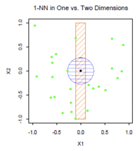
As dimension grows the concept of locality gets thin.
(source: Elements of Statistical Learning)
Data is distributed along the boundary
Let $\mathbf{X} = (X_1,\cdots,X_p)$ be a random vector from uniform distribution over a $p$-dimensional unit ball, centered at $\mathbf{0}.$ Let $R_i = \sqrt{\sum_{k=1}^p X_{ki}^2}$ be the distance of $\mathbf{X}_ i.$ Let $R_ {(1)}$ be the smallest of $R_1,\cdots,R_N.$ Then
\[\begin{aligned} \mathbb{P}(R_i < r) &= r^p/1^p = r^p,~~ 0\le r\le 1.\\ \mathbb{P}(R_{(1)} < r) &= \sum_{j=1}^N {N \choose j} (r^p)^j (1-r^p)^{N-j} \\ &= (r^p + 1 - r^p)^N - {N \choose 0}(r^p)^0 (1-r^p)^N. \end{aligned}\]Then the median $r$ of the distribution of $R_{(1)}$ is
\[\begin{aligned} &\mathbb{P}(R_{(1)} < r) = \frac{1}{2} \\ &\iff 1 - (1 - r^p)^N = \frac{1}{2} \\ &\iff (1-r^p)^N = \frac{1}{2} \\ &\iff 1 - r^p = \left(\frac{1}{2}\right)^{1/N} \\ &\iff r = \left(1 - \left(\frac{1}{2}\right)^{1/N}\right)^{1/p}. \end{aligned}\]Thus for $N=5000,$ $p=10,$ $r\approx0.52.$ This means more than half of the data is closer to the boundary than the center.
Bias increases as dimension grows
Suppose the true model is deterministic:
\[y = e^{-8\|\mathbf{X}\|^2}.\]Consider the $1$-NN model at $x=0,$ then
\[\text{bias} = 1-e^{-8\|\mathbf{X}_{(1)}\|^2},~~ \mathbf{X}_1 \in \mathcal{L},\]where $\mathcal{L}$ is the training data. Since the data gets closer to boundary as dimension increases, the bias increases as $p$ increases. This makes k-NN model impractical in high dimensional problems.
Overfitting
In the regression problem, since EPE cannot be computed, we try to estimate it using training error (TE). However, training error underestimates EPE because the training data $\mathcal{L}$ is used in both model building and TE calculation. In addition, TE monotonically decreases while EPE does not. This phenomenon in which EPE increases even though the TE decreses is called overfitting.
Overfitting can be viewed as bias-variance trade-off. Suppose our true model is
\[Y = f(X) + \epsilon,~ E\epsilon=0,~ \text{Var}(\epsilon)=0.\]where $\epsilon \perp X,\mathcal{L}$ and $f(X, \mathcal{L})$ is our trained model. Then the training error $\text{TE}$ is
\[\begin{aligned} \text{TE}~ =&~ E_\mathcal{L}E_{(X,Y)} \big( Y - f(X, \mathcal{L}) \big)^2 \\ =&~ E_\mathcal{L}E_{(X,Y)} \big( Y - f(X) + f(X) - E_\mathcal{L}f(X, \mathcal{L})+E_\mathcal{L}f(X, \mathcal{L}) - f(X,\mathcal{L}) \big)^2 \\ =& E_{(X,Y)} \big(Y-f(X)\big)^2 + E_X\big(f(X)-E_\mathcal{L}f(X,\mathcal{L})\big)^2 + E_\mathcal{L}E_{(X,Y)} \big(E_\mathcal{L}f(X,\mathcal{L}) - f(X,\mathcal{L})\big)^2 \\ &+2\big\{ \underbrace{E_{(X,Y)}\big[(Y-f(X))(f(X) - E_\mathcal{L}f(X,\mathcal{L}))\big]}_{\text{(1)}} \\ &+\underbrace{E_\mathcal{L}E_{(X,Y)} \big[ (f(X) - E_\mathcal{L}f(X,\mathcal{L}))(E_\mathcal{L}f(X,\mathcal{L}) - f(X, \mathcal{L})) \big]}_{\text{(2)}} \\ &+ \underbrace{E_\mathcal{L}E_{(X,Y)} \big[ (Y-f(X))(E_\mathcal{L}f(X,\mathcal{L}) - f(X,\mathcal{L})) \big]}_{\text{(3)}} \big\}. \end{aligned}\]where
\[\begin{aligned} \text{(1)} &= E_XE_{Y|X} \big[\epsilon (f(X) - E_\mathcal{L}f(X,\mathcal{L}))\big] \\ &= (E_{Y|X} \epsilon ) \cdot E_X\big[ f(X) - E_\mathcal{L}f(X,\mathcal{L}) \big] \\ &= 0,\\ \text{(2)} &= E_X \left[ \big( f(X) - E_\mathcal{L}f(X,\mathcal{L}) \big) \cdot \cancel{E_\mathcal{L}\big[ E_\mathcal{L}f(X, \mathcal{L}) - f(X, \mathcal{L}) \big]} \right] \\ &=0, \\ \text{(3)} &= E\left[ \epsilon \cdot \big( E_\mathcal{L}f(X, \mathcal{L}) - f(X, \mathcal{L}) \big) \right] \\ &= E\epsilon \cdot \big( E_\mathcal{L}f(X, \mathcal{L}) - E_\mathcal{L}f(X, \mathcal{L}) \big) \\ &=0. \end{aligned}\]Thus
\[\text{TE} = \sigma^2 + E_X \text{bias}_\mathcal{L}^2(f\big(X,\mathcal{L})\big) + E_X \text{Var}_\mathcal{L}\big( f(X,\mathcal{L}) \big).\]As the model complexity increases, bias decreases but variance increases, which indicates overfitting. In the case of k-NN, let $X_{(i)}$ be the $i$-th closest neighbor. Then
\[\begin{aligned} \text{bias}_\mathcal{L}(f\big(X,\mathcal{L})\big) &= f(x) - \frac{1}{k}\sum_{i=1}^k f(X_{(i)}), \\ \text{Var}_\mathcal{L}\big( f(X,\mathcal{L}) \big) &= \frac{1}{k}\sigma^2. \end{aligned}\]Thus as $k$ decreases (i.e. complexity $\uparrow$), bias decreases but variance increases.
References
- Hastie, Tibshirani, Friedman. 2008. The Elements of Statistical Learning. 2nd edition. Springer.
- Advanced Data Mining (Spring, 2021) @ Seoul National University, Republic of Korea (instructor: Prof. Yongdai Kim).