Understanding Restricted Boltzmann Machine
A Boltzmann machine is an unsuperviced generative model that learns the probability distribution of a random variable using the Boltzmann distribution. Although it has been proposed in 1985, practical utilization was nearly impossible for samples of nontrivial sizes. Only later in 2002 when the restricted version of it overcame the implausibility did it became a widely used algorithm.
Boltzmann machine
We will consider the simplest version here: The one without any hidden units.
Let $\mathbf x=(x_1,\cdots,x_m)^\intercal \in \mathbb \{0, 1\}^m$ be a realization of a binary $m$-dimensional random vector following the distribution $P.$ Each entry $x_i$ will become a unit (node) of the network (Boltzmann machine) that is visible (observable). One can interpret that the unit $x_i$ is “on” if $x_i=1$ and is “off” otherwise. Suppose that we have a training data $\{\mathbf x_\ell:~ 1\le \ell\le L\}$ of size $L.$ Our goal is to learn $p$ using the data at hand. A (unrestricted) Boltzmann machine (BM) models the distribution with the Boltzmann distribution with product of Boltzmann constant $k$ and temperature $T$ set to $kT=1$ and the energy $E(\mathbf x)$ of the visible (observed) sample $\mathbf x$ follows the formula below.
\[\hat p(\mathbf x) = \frac {e^{-E(\mathbf x)}} Z,~~ Z=\sum_{\mathbf x} e^{-E(\mathbf x)},\] \[E(\mathbf x) = \color{blue}{ -\sum_{1\le i<j\le m} w_{ij}x_ix_j } \color{green}{ -\sum_{i=1}^m a_ix_i } \tag{1}\label{1}\]where $w_{ij}$ is the strength of connection between the $i$th element and the $j$th element and $a_i$ is a threshold. I would like to comment on the three main concepts regarding the model.
1. Strength of connection
In Boltzmann machine setting, we assume that $w_{ij}=w_{ji}$ which makes it a symmetric Hopfield network. This can be represented as a graph.
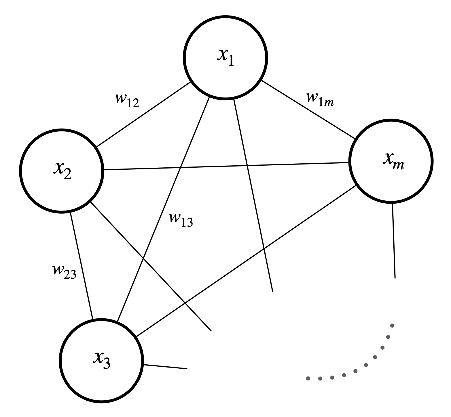
Figure 1. A Boltzmann machine with visible units only
2. Energy
The energy $E(\mathbf x)$ is assigned to each global state of the network. I will directly quote Wikipedia for the rationale behind the naming “energy”. If you are interested in the original explanation, see Hopfield (1982).
This quantity is called “energy” because it either decreases or stays the same upon network units being updated. Furthermore, under repeated updating the network will eventually converge to a state which is a local minimum in the energy function. (…) Thus, if a state is a local minimum in the energy function it is a stable state for the network. (Hopfield network, Wikipedia)
Hopfield (1982) derived a local minimizer as follows.
\[\begin{cases} w_{ij} = \frac1L \sum_{\ell=1}^L x_{\ell i} x_{\ell j} \\ a_i = \frac1L \sum_{\ell=1}^L x_{\ell i} \end{cases}\]For the Hopfield solution, the suggestion of such energy formula follows from the Hebb’s rule, which is a neuroscientific theory that accounts for neuronal plasticity. The punchline of the rule is that “neurons wire together if they fire together”. This is because $w_{ij}$ is a sample correlation and $a_i$ is a sample mean of $\mathbf x_\ell$:
\[\begin{aligned} \color{blue}{ \sum_{1\le i<j\le m} w_{ij}x_ix_j } ~&\text{increases as the sample correlation $w_{ij}$} \\ &\text{and the correlation of an unseen sample $x_ix_j$ coincides}\\ \color{green}{ \sum_{i=1}^m a_ix_i } ~&\text{increases as the sample mean $a_i$} \\ &\text{and the value of an unseen sample $x_j$ coincides} \end{aligned}\]3. Threshold
Define the local energy $E(x_k) := -\sum_{i}w_{ki}x_kx_i - a_kx_k$ at the $k$-th unit. Then in the symmetric connection setting, the energy gap at the $k$-th unit is computed as
\[\Delta E(x_k) = E(x_k=0)-E(x_k=1) = \sum_i w_{ki}x_i + a_k.\]Notice that during the learning process, the model tends to turn the $k$-th unit on if the surrounding signal $\sum_i w_{ki}x_i$ of the unit $x_k$ is stronger than the value $\theta_k:=-a_k.$ This is why we call the term “threshold” (Ackley et al., 1985).
Learning process
Let $p_L$ be the empirical density (or mass) based on $L$ observations and $\hat p$ be the candidate that the machine learned. To find $w_{ij}$ and $a_i$ that minimizes the deviation of $\hat p$ from the true density $p,$ Ackley et al. (1985) chose the Kullback-Leibler divergence of $p_L$ from $\hat p$ as the objective function. It is clear that if $\hat p(\mathbf x) = p_L(\mathbf x)$ then $K(\hat p| p_L)$ so it makes sense.
\[\begin{aligned} K(p_n\|\hat p) &= \sum_\mathbf{x} p_L(\mathbf x) \log\frac{p_L(\mathbf x)}{\hat p(\mathbf x)} \\ &= -\sum_\mathbf{x} p_L(\mathbf x)\log \hat p(\mathbf x) + \sum_\mathbf{x} p_L(\mathbf x) \log p_L(\mathbf x) \\ &= \mathbb E_{\{\mathbf x_\ell\}_{\ell=1}^L} \left[\log \frac1{\hat p(\mathbf x)}\right] - \mathbb E_{\{\mathbf x_\ell\}_{\ell=1}^L} \left[\log \frac1{p_L(\mathbf x)}\right] \end{aligned}\]Note that the logarithm of inverse of density can be thought of information. Similar to how we named mutual information, we can name this a relative information.
Using the gradient descent algorithm, we get the update rule
\[w_{ij} \leftarrow w_{ij} - \lambda \frac{\partial K}{\partial w_{ij}}\\ a_i \leftarrow a_i - \lambda \frac{\partial K}{\partial a_i}\]where $\lambda$ is the predefined learning rate and
\[\begin{aligned} -\frac{\partial K}{\partial a_i} &= \frac{\partial}{\partial a_i} \sum_\mathbf{x} p_L(\mathbf x)\log \hat p(\mathbf x) \\ &= \frac{\partial}{\partial a_i} \sum_\mathbf{x} p_L(\mathbf x) (-E(\mathbf x) - \log Z) \\ &= \sum_{\mathbf x} p_L(\mathbf x)x_i - \frac1Z \frac{\partial Z}{\partial a_i} \\ &= \sum_{\mathbf x} p_L(\mathbf x)x_i - \sum_{\mathbf x} \hat p(\mathbf x)x_i \\ &= \mathbb E_{\{\mathbf x_\ell\}_{\ell=1}^L} [x_i] - \mathbb E_{\hat p}[x_i]. \end{aligned}\]Similarly, the gradient with respect to $w_{ij}$ is
\[-\frac{\partial K}{\partial w_{ij}} = \mathbb E_{\{\mathbf x_\ell\}_{\ell=1}^L} [x_i x_j] - \mathbb E_{\hat p}[x_i x_j].\]Implausibility
Notice that computation of gradients require summation over all possible values of $\mathbf x.$ Consider the famous MNIST dataset as an example. Suppose that each pixel has either 0 or 1 as its value. Then a single 28$\times$28 image $\mathbf x$ can have $2^{28\times28}$ different values. Summation of $2^{784}$ is implausible even for a high performant computer.
Restricted Boltzmann Machine
It is quite discouraging that the model is implausible even for a not-so-big data. Follow up research was mainly focused on constraints makes the model plausible for data of nontrivial size while maintaining its theoretical advantages. Hinton (2002) proposed the one: the restricted Boltzmann machine (RBM).
Consider a BM with hidden nodes (nodes that cannot be observed). Hinton thought of a BM as a network between layers of units. RBM restricts the ordinary Boltzmann machine by imposing a constraint that each node within the same layer cannot have connections.

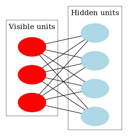
Figure 2. (left) A Boltzmann machine with visible units (white) and hidden units (blue). (right) A restricted Boltzmann machine. (Sources: left, right)
Under this constraint, the visible unit $x_i$ can have relationship with $x_j$ only through the hidden (latent) unit $h_k.$ In this sense the hidden unit $\mathbf h$ can be interpreted as the internal representation of $\mathbf x$.
Now, as in the ordinary BM, we have a learned density $\hat p$ but this time it is a joint density of $(\mathbf x, \mathbf h).$
\[\hat p(\mathbf x, \mathbf h) = \frac{e^{-E(\mathbf x, \mathbf h)}}Z,~ Z=\sum_{\mathbf x, \mathbf h} e^{-E(\mathbf x, \mathbf h)}\]where joint energy is defined similar to $\eqref{1}$ as well.
\[E(\mathbf x, \mathbf h) = -\sum_{i,j} w_{ij}x_ih_j -\sum_{i} a_ix_i -\sum_{j} b_jh_j\]Notice the additional threshold $\mathbf b$ for hidden units $\mathbf h$ and the correlation is now in between $\mathbf x$ and $\mathbf h.$ Estimation of the marginal $p_L(\mathbf x)$ is done by marginalizing the joint density over $\mathbf h$: $\hat p_\mathbf{X}(\mathbf x) = \sum_{\mathbf h} \hat p(\mathbf x,\mathbf h).$
Activation probabilities of hidden units
There are some additional assumptions from the model structure. We assume that, by the restriction on connection between units in the same layer, activation of hidden units ($h_j$’s) are mutually independent given observable units ($x_i$’s). That is,
\[x_i|\mathbf h \overset{\text{i.i.d.}}{\sim} \text{Multinomial},~ 1\le i\le m \\ h_j|\mathbf x \overset{\text{i.i.d.}}{\sim} \text{Bernoulli},~ 1\le j\le n\]From this activation probabilities are direct:
\[\begin{cases} \hat p_{\mathbf H|\mathbf X}(h_{j}=1|\mathbf x) + \hat p_{\mathbf H|\mathbf X}(h_{j}=0|\mathbf x) = 1, \\ \frac{\hat p_{\mathbf H|\mathbf X}(h_{j}=1|\mathbf x)}{\hat p_{\mathbf H|\mathbf X}(h_{j}=0|\mathbf x)} = \frac{e^{-E(h_j=1)}/\cancel Z}{e^{-E(h_j=0)}/\cancel Z} = e^{\Delta E(h_j)}. \end{cases}\tag{2}\label{2}\]where
\[\begin{aligned} \Delta E(h_j) &= E(\mathbf x,h_j=0)-E(\mathbf x,h_j=1) \\ &= \sum_i w_{ij}x_i + b_j. \end{aligned}\]Solving the equation $\eqref{2}$ yields
\[\hat p_{\mathbf H|\mathbf X}(h_j=1|\mathbf x) = \frac{e^{\Delta E(h_j)}}{1 + e^{\Delta E(h_j)}} = \sigma\left( \sum_i w_{ij}x_i + b_j \right) \\ \hat p_{\mathbf H|\mathbf X}(h_j=0|\mathbf x) = \frac 1 {1 + e^{\Delta E(h_j)}} = \sigma\left( -\sum_i w_{ij}x_i - b_j \right) \tag{3}\label{3}\]These activation probabilities will be later used in Gibbs sampling step.
Minimizing the KL divergence
The scheme of the learning process is more or less the same as in an ordinary BM: We find the minimizer of the KL divergence $K=K(p_L\|\hat p_\mathbf{X})$. In fact, since the $p_L$ part is fixed, it is equivalent to minimize the negative log likelihood $-\log \hat p_\mathbf{X}(\mathbf x).$ In this equivalent problem, the gradient descent update rule becomes
\[w_{ij} \leftarrow w_{ij} - \lambda \frac{\partial}{\partial w_{ij}} \left(-\log \hat p_{\mathbf X}(\mathbf x)\right) \\ a_i \leftarrow a_i - \lambda \frac{\partial}{\partial a_i} \left(-\log \hat p_{\mathbf X}(\mathbf x)\right) \\ b_i \leftarrow b_i - \lambda \frac{\partial}{\partial b_i} \left(-\log \hat p_{\mathbf X}(\mathbf x)\right)\]Gradients can be computed as follows. Below, the placeholder $\theta$ can be replaced to any parameters being updated ($a_i$, $b_j$, or $w_{ij}$).
\[\begin{aligned} &\frac{\partial}{\partial \theta} \left(-\log \hat p_{\mathbf X}(\mathbf x)\right) \\ &= \frac{\partial}{\partial \theta} \left(-\log \sum_{\mathbf h} \hat p(\mathbf x, \mathbf h)\right) \\ &= \frac{\partial}{\partial \theta} \left[ \log\left(\sum_{\mathbf x, \mathbf h}e^{-E(\mathbf x, \mathbf h)}\right) - \log\left(\sum_{\mathbf h}e^{-E(\mathbf x, \mathbf h)}\right) \right] \\ &= -\frac1{\left(\sum_{\mathbf x, \mathbf h}e^{-E(\mathbf x, \mathbf h)}\right)} \left(\sum_{\mathbf x, \mathbf h}e^{-E(\mathbf x, \mathbf h)}\right) \frac{\partial}{\partial \theta}E(\mathbf x, \mathbf h) \\ &\;\;\;\;+ \frac1{\left(\sum_{\mathbf h}e^{-E(\mathbf x, \mathbf h)}\right)} \left(\sum_{\mathbf h}e^{-E(\mathbf x, \mathbf h)}\right) \frac{\partial}{\partial \theta}E(\mathbf x, \mathbf h) \\ &=-\sum_{\mathbf x, \mathbf h} \hat p(\mathbf x, \mathbf h) \frac{\partial}{\partial\theta} E(\mathbf x, \mathbf h) + \sum_{\mathbf h} \hat p_{\mathbf H|\mathbf X}(\mathbf h|\mathbf x) \frac{\partial}{\partial\theta} E(\mathbf x, \mathbf h) \\ &=-\color{blue}{ \mathbb E_{\hat p} \left( \frac{\partial}{\partial\theta}E(\mathbf x, \mathbf h) \right) } + \color{green}{ E_{\hat p_{\mathbf H|\mathbf X}}\left( \frac{\partial}{\partial\theta} E(\mathbf x, \mathbf h) \right) } \end{aligned}\]In some literature the blue part is referred to as the negative gradient and the green part as the positive gradient. Since
\[\begin{cases} \frac{\partial}{\partial w_{ij}} E(\mathbf x, \mathbf h) = -x_ih_j \\ \frac{\partial}{\partial a_i} E(\mathbf x, \mathbf h) = -h_j\\ \frac{\partial}{\partial b_j} E(\mathbf x, \mathbf h) = -x_i \end{cases}\]by replacing the placeholder $\theta,$ the gradient becomes
\[\begin{aligned} &\frac{\partial}{\partial w_{ij}}\left(-\log \hat p_{\mathbf X}(\mathbf x)\right) \\ &= \color{blue}{ \sum_{\mathbf x, \mathbf h} \hat p(\mathbf x, \mathbf h) x_ih_j } - \color{green}{ \sum_{\mathbf h} \hat p_{\mathbf H|\mathbf X}(\mathbf h|\mathbf x) x_ih_j } \end{aligned}\]Here, the positive gradient (blue term) can be interpreted as the probability density of the input data, and the negative one (green term) can be interpreted as the learned probablity density. It is quite similar to the form of the gradients in ordinary BM model.
During the training process, the second term can be computed asymptotically by Gibbs sampling. Detail will be covered in the next subsection.
Learning process
Synthesizing all the results from earlier subsections, we arrive at the learning process of a RBM.
Repeat the following until convergence of parameters for the training data.
- Take a sample $\mathbf x$ from the training data. Compute $\hat p_{\mathbf H|\mathbf X}(h_j|\mathbf x)$ using the equation $\eqref{3}$.
- Compute the gradient.
- Compute positive gradient: $\mathbf x \mathbf h^\intercal$.
- Apply Gibbs sampling:
- Sample $\tilde {\mathbf x}$ from $\mathbf h.$
- Sample $\tilde {\mathbf h}$ from $\tilde{\mathbf x}.$
- Compute negative gradient: $\tilde{\mathbf{x}} \tilde{\mathbf{h}}^\intercal$
- Update parameters.
- $\Delta \mathbf W = \mathbf x \mathbf h^\intercal - \tilde{\mathbf{x}} \tilde{\mathbf{h}}^\intercal$
- $\Delta\mathbf a = \mathbf x - \tilde{\mathbf x}$
- $\Delta\mathbf b = \mathbf h - \tilde{\mathbf h}$
Relation of RBM to neural nets
One might notice that the RBM closely resembles the structure of a neural net. In fact, the forward feeding of a RBM can be viewed as a forward propagation of a stochastic neural net with sigmoid function $\sigma$ as its activation function that only have binary outputs. That is, recall the equation
\[\hat p_{\mathbf H|\mathbf X}(h_j=1|\mathbf x) = \sigma \left( \sum_{i} w_{ij}x_i + b_j \right).\]References
- Hopfield. 1982. Neural Networks and Physical Systems with Emergent Collective Computational Abilities. Proceedings of the National Academy of Sciences of the United States of America. 79 (8): 2554-2558.
- Ackley, Hinton and Sejnowski. 1985. A learning Algorithm for Boltzmann Machines. Cognitive Science. 9 (1): 147-169.
- Hinton. 2002. Training Products of Experts by Minimizing Contrastive Divergence. Neural Computation. 14 (8): 1771-1800.
- Choi. 2018. 논문으로 짚어보는 딥러닝의 맥.
- The 12th KIAS CAC Summer School, Korea Institute for Advanced Study, Republic of Korea (the talk was given by Prof. Junghyo Jo at Seoul National Univerisity).