3. Shrinkage Estimators
As a remedy for overdetermined systems and variable selection rule, I would like to cover shrinkage methods in this section. Especially, I would like to focus on ridge and lasso penalization.
Variable selection
We want to have a model without colinearity that can be generalized into unseen data as well. As Occam’s razor states, it is helpful to select only subsets among total of $p$ variables.
For this, we repeat the following for all $0\le k\le p.$
- Select the best set among possible choices of $k$ variables, and let the model $M_k$ be the one that used it.
Then select the best performing model $M^*_k \in \{M_k: 0\le k\le p\}.$ This is a straightforward selection method, but as $\sum_{k=0}^p{p \choose k} = 2^p$ fitting of linear models is required, it is computationally inefficient. In addtion, since we either use a variable or not, it is a hard decision rule (or hard-thresholding) which makes the method unstable: small changes in the data leads to large change in estimator.
Ridge estimator
Ridge estimator can be seen as a soft decision rule. That is, it does not entirely drops a subset of variables, but rather gives weights to variables (proportional shrinkage). It tends to give more stable and better cross-validation results than variable selection methods. Ridge estimator for linear regression can be derived as
\[\hat{\boldsymbol\beta}^\text{ridge} = \argmin_{\boldsymbol\beta} \sum_{i=1}^n \left( y_i - \beta_0 - \sum_{k=1}^p x_i^\intercal \beta_k \right)^2 \text{ subject to } \sum_{k=1}^p \beta_k^2 \le t.\]This constrained form is equivalent to the penalized form below.
\[\hat{\boldsymbol\beta}^\text{ridge} = \argmin_{\boldsymbol\beta} \left[ \sum_{i=1}^n\left(y_i - \beta_0 - \sum_{k=1}^p x_i^\intercal \beta_k\right)^2 + \lambda \sum_{k=1}^p \beta_k^2 \right].\]The latter form is more computationally efficient. In fact, we can easily derive closed form solution.
Notice that if the squared norm of the ordinary least squares estimator (LSE) is large so that $\| \hat{\boldsymbol\beta}^\text{LS} \| > t,$ then $\beta_k^\text{LS} > \beta_k^\text{ridge}$ and otherwise $\beta_k^{LS} = \beta_k^\text{ridge}.$ Thus we can say that the ridge penalization shrinks the LS estimator towards zero.
Motivation to shrinkage estimator
There are several motivation for the estimator that “shrinks” the ordinary LS estimator toward some other value (mostly zero).
1. To achieve nonsingular Gram matrix
$X^\intercal X$ is refered to as the Gram matrix. Since the LS estimator is
\[\hat{\boldsymbol\beta}^\text{LS} = (X^\intercal X)^{-1}X^\intercal Y,\]we need invertibility of $X^\intercal X$, or equivalently full ranked $X \in \mathbb{R}^{n\times p}.$ However in high dimensional setting, often the number of variables $p$ is larger than $n,$ which makes $X^\intercal X$ singular.
Hoerl and Kennard (1970) came up with the simple solution: make $X^\intercal X$ invertible by adding a constant $\lambda$ to diagonal elements. That is, replace $X^\intercal X$ by $X^\intercal X + \lambda I$ to get the estimator
\[\hat{\boldsymbol\beta} = (X^\intercal X + \lambda I)^{-1}X^\intercal Y.\]This is the original derivation of ridge estimator.
2. James-Stein estimator
Another motivation is that in cases where $p \ge 3,$ shrinkage estimator actually performs better in terms of MSE.
Suppose we want to estimate $\boldsymbol{\theta}$ with a single sample
\[\mathbf{X} = (X_1,\cdots,X_p) \sim \mathcal{N}_p(\boldsymbol{\theta}, \sigma^2 I).\]Note that the MLE is $\mathbf{X}.$ However, unintuitively, $X$ is suboptimal if $p \ge 0.$ This phenomenon is called Stein’s paradox. James and Stein independently proved that there exists a better estimator
\[\delta^\text{JS} = \left(1 - \frac{1}{\sum_{i=1}^p X_i^2}\right) \mathbf{X}.\]Since we can safely assume that $\sum_{i=1}^p X_i^2 > 1$ for large $p,$ the James-Stein estimator $\delta^\text{JS}$ can be viewed as a shrinkage estimator that shrinks $\mathbf{X}$ toward zero.
3. Bayesian perspective
Last but not least, ridge estimator can be explained as a maximum a posteriori (MAP) estimator in Bayesian framework. Assume that $X$ and $\sigma^2$ and $\tau^2$ are known and fixed. Consider a Bayesian setting that gives normal prior to $\boldsymbol\beta.$
\[Y = X{\boldsymbol\beta} + \epsilon,~ \epsilon \sim \mathcal{N}_n(0, \sigma^2I).\\ {\boldsymbol\beta} \sim \mathcal{N}_p(0, \tau^2I).\]Then
- likelihood: $(Y|{\boldsymbol\beta}) \sim \mathcal{N}_n(X{\boldsymbol\beta},\sigma^2I).$
- posterior: $({\boldsymbol\beta}|Y) \propto p(Y|{\boldsymbol\beta})p({\boldsymbol\beta}).$
Hence the MAP estimator maximizes the log posterior
\[\hat{\boldsymbol\beta}^\text{MAP} = \argmax_{\boldsymbol\beta} \left[ \sum_{i=1} \frac{1}{2\sigma^2}\left( y_i - \beta_0 - \sum_{k=1}^p x_k\beta_k \right)^2 + \frac{1}{\tau^2} \sum_{k=1}^p \beta_k^2 \right]\]which is the same formulation as in penalized form of ridge estimator with $\lambda = \tau^2/\sigma^2.$
Ridge logistic regression
Logistic regression with ridge penalization can be defined in a similar way.
\[\hat{\boldsymbol\beta}^\text{ridge} = \argmax_{\boldsymbol\beta} \left[ \sum_{i=1}^n \left( -y_i(\beta_0 + x_i^\intercal {\boldsymbol\beta} - \log(1 + e^{\beta_0 + x_i^\intercal {\boldsymbol\beta}}) \right) + \lambda \sum_{k=1}^p \beta_k^2 \right].\]We use IRLS as in unconstrained problem for optimization.
LASSO estimator
While ridge provide more robust estimator than LS estimator, it does not actually “select” a subset of variables. Tibshirani (1996) proposed a penalization that selects and shrinks the LS estimate simultaneously. He called it a LASSO (least absolute shrinkage and selection operator) estimator. Lasso is simply replaces $\ell^2$-norm penalty from ridge objective function with $\ell^1$-norm penalty.
\[\begin{aligned} &\text{minimize } \sum_{i=1}^n \ell(y_i, x_i^\intercal \boldsymbol\beta) \\ &\text{subject to } \sum_{k=1}^p |\beta_k| \le t \end{aligned}\]This is equivalent to
\[\text{minimize } \sum_{i=1}^n \ell(y_i, x_i^\intercal \boldsymbol\beta) + \lambda \sum_{k=1}^p |\beta_k|.\]Note that unlike ridge, lasso objective function is non-differentiable with respect to $\beta_k$’s’ at $\beta_k = 0.$ This property of lasso tends to makes it produce a sparse model, i.e. a model with values of many $\beta_k$ is equal to zero. For simplicity of explanation, consider a model with $p=2$ variables $Y = \beta_0 + \beta_1 x_1 + \beta_2x_2.$
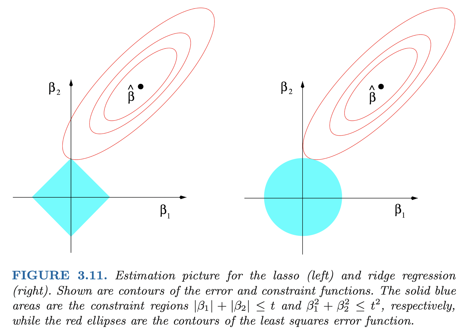
(source: Elements of Statistical Learning)
Then the constraint region of lasso becomes a diamond $|\beta_1| + |\beta_2| \le t,$ which has corners. Since constraint optimization problem is to find the point that the objective function contour first touches the constrain region, lasso optimum is highly likely to be placed at one of the corners of the diamond. Since the corner implies one (or more, in $p \ge 3$ case) of $\beta_k$’s, this makes it produce a sparse model.
If sparsity is the only important property, then why don’t we use other $\ell^q$-norm penalties with $0<q<1$? In fact there is another property that makes optimization problem fairly easy. Ridge and lasso constraints are convex. In optimization problem of convex objective function, first order optimality condition is sufficient for local optima searching, which makes the problem super efficient. It can be easily shown that the lasso penalty is the only $\ell^q$-norm penalty that is both convex and non-differentiable at the corners.
Similar to ridge estimator, lasso estimator can be justified as a Bayesian MAP estimator with double exponential prior given to $\boldsymbol\beta.$
Optimization of LASSO problems
Optimization of lasso objective function can be formed as a quadratic program (QP). Here, we first cover the essentials of convex optimization theory, and then describe details of three optimization algorithms for lasso problems.
Essentials of convex optimization
Consider the minimization problem
\[\begin{aligned} \text{minimize } ~&f(\mathbf{x}) \\ \text{subject to } ~&h(\mathbf{x})=0, \\ &g(\mathbf{x}) \le 0 \end{aligned} \tag{P}\]where $f:\mathcal{X}\to\mathbb{R},$ $h=(h_1,\cdots,h_m):\mathcal{X} \to \mathbb{R}^m,$ $g=(g_1,\cdots,g_r):\mathcal{X} \to \mathbb{R}^r.$
We call it a convex optimization if $f$ is convex and $h_i, g_j$ are linear for all $i,j.$ Furthermore, we call it a quadratic program (QP) if $f$ is a quadratic function in particular.
We can easily show that the lasso problem with $\ell^2$-type objective function is a QP.
$$ \begin{aligned} \text{minimize } & \|Y-X\boldsymbol\beta\|_2^2 \\ \text{subject to } & \|\boldsymbol\beta\|_1 \le t \\ \iff \text{minimize } & \|Y-X\boldsymbol\beta\|_2^2 \\ \text{subject to } & \sum_{k=1}^p \beta_k^+ + \sum_{k=1}^p \beta_k^- \le t, \\ & \beta_k^+ \ge 0,~ \beta_k^- \ge 0,~ k=1,\cdots,p. \end{aligned} $$
From now on, we assume that the problem (P) is a convex optimization.
The problem (P) defined above is called the primal problem.
\[L(\mathbf{x}, \lambda, \mu) := f(\mathbf{x}) + \lambda^\intercal h(\mathbf{x}) + \mu^\intercal g(\mathbf{x})\]is the Lagrangian form of the problem (P), where $\lambda \in \mathbb{R}^m$ and $\mu \in \mathbb{R}^r.$
Suppose $\mathbf{x}^*$ be the optimum of the problem. For the $j$-th equality constraint, if the inequality is strict
\[g_j(\mathbf{x}^*) < 0,\]then this constraint is not actually limiting the optimum of objective function $x^*$ to be inside of the constraint region. We collect inequality constraints that achieves the boundary (zero) at a point $\mathbf{x}$ and call it active contraints $A(\mathbf{x})$ at $\mathbf{x}$.
\[A(\mathbf{x}) := \{j: g_j(\mathbf{x})=0\}.\]In addition, in many cases gradients $\nabla h_i(\mathbf{x}),$ $i=1,\cdots,m$ at $\mathbf{x}$ need to be linearly independent since otherwise $\mu$ is not identifiable. Similarly, $\nabla_j g_j(\mathbf{x})$ need to be linearly independent as well. If the point $\mathbf{x}^*$ satisfies these linearly independent gradient conditions, then we call $\mathbf{x}^*$ a regular point.
Now we discuss our first theorem: the Karuch-Kuhn-Tucker (KKT) necessary conditions.
$\implies$ There uniquely exist $\lambda^*$ and $\mu^*$ that satisfies the followings.
(i) (stationarity) $\nabla_\mathbf{x} L(\mathbf{x}^*, \lambda^*, \mu^*) = 0.$
(ii) (primal feasibility) $g(\mathbf{x}^*)\le0,$ $h(\mathbf{x}^*)=0.$
(iii) (dual feasibility) $\mu^* \ge 0.$
(iv) (complementary slackness) $\mu^{*\intercal} g(\mathbf{x}^*) = \mathbf{0}.$
KKT necessary condition can be viewed as the first order optimality condition for constrained optimization problem. The next theorem is a second order sufficient condition for constrained problem.
(i) (stationarity) $\nabla_\mathbf{x} L(\mathbf{x}^*, \lambda^*, \mu^*) = 0.$
(ii) (primal feasibility) $g(\mathbf{x}^*)\le0,$ $h(\mathbf{x}^*)=0.$
(iii) (strict complementarity) $\mu_j>0$ for $j\in A(\mathbf{x}^*)$ and $\mu_j=0$ for $j \notin A(\mathbf{x}^*).$
(iv) (convex point) $\mathbf{s}\ne \mathbf{0},$ $\nabla h(\mathbf{x}^*)^\intercal\mathbf{s}=0,$ $\left[\nabla g_j(\mathbf{x}^*)\right]_{j\in A(\mathbf{x}^*)}^\intercal \mathbf{s} = 0$ $\implies$ $\mathbf{s}^\intercal \nabla_{\mathbf{x}\mathbf{x}}^2 L(\mathbf{x}^*,\lambda^*, \mu^*) \mathbf{s} > 0.$
We will also use Lagrangian duality later, so let’s define it here.
$$ g(\lambda, \mu) := \inf_{\mathbf{x}\in\mathcal{X}} L(\mathbf{x}, \lambda, \mu) $$ is the Lagrangian of the problem (P). The dual problem of (P) can be formed as $$ \begin{aligned} \text{maximize } & g(\lambda, \mu) \\ \text{subject to } & \mu \ge 0 \end{aligned} \tag{D} $$
Note that the dual problem is a maximization problem. Under some conditions, we can show that solving the dual problem (D) is equivalent to solving the primal (P). This is called the duality theorem.
(i) (primal feasibility) $g(\mathbf{x}^*) \le 0,$ $h(\mathbf{x}^*)=0$.
(ii) (dual feasibility) $\mu^* \ge 0.$
(iii) (complementary slackness) $\mu^{*\intercal}g(\mathbf{x}^*)=0.$
(iv) (local optimality) $\mathbf{x}^* \in \{\mathbf{x}: \argmin_\mathbf{x}L(\mathbf{x}, \lambda^*, \mu^*)\}.$
Why consider dual problem? Because it can be shown that dual problems are always convex optimization regardless of the primal problem. In addition, it is often much easier to solve the problem with respect to $\lambda$ and $\mu.$
Solution path algorithm
[TBD]
References
- Hastie, Tibshirani, Friedman. 2008. The Elements of Statistical Learning. 2nd edition. Springer.
- Advanced Data Mining (Spring, 2021) @ Seoul National University, Republic of Korea (instructor: Prof. Yongdai Kim).