2. Linear classifiers
In this chapter, linear classifiers will be introduced and will be compared. Specifically, logistic regression and linear discriminant analysis will be described in detail.
- Linear classifiers
- Linear discriminant analysis
- Logistic regression
- Extension to multi-class problem
Linear classifiers
Here, our setting will be binary classification problem. That is,
\[\mathcal{Y}=\{0,1\} \text{ or } \{-1,1\},\\ \ell(y,a) = \mathbf{1}(y\ne a).\]Linear model assumes linear decision boundary:
\[\{x: \beta_0 + x'\boldsymbol{\beta} = 0\}.\]Under this decision boundary, our classifier $G: \mathbb{R}^p \to \mathcal{Y}$ will be
\[G(x) = \text{sign}\big(f(x)\big),~ f(x)=\beta_0 + x'\boldsymbol{\beta}.\]Descriptive vs. generative model
Descriptive model models $\mathbb{P}(y|x),$ while generative model models both $\mathbb{P}(x|y)$ and $\pi(y)$ which makes it possible to model the joint probability $\pi(x,y).$ While descriptive model generally requires less assumptions and performs better, generative model can “generate” the data according to modeled joint probability, thus more explainable and useful in semi-supervised settings.
Linear discriminant analysis
Linear discriminant analysis, or LDA, is a generative approach to classification. It assumes the density of $x$ given $y=j$ to be that of normal distribution. i.e.
\[f_j(x) = p(x|Y=j) := \phi_{(\mu_j, \Sigma_j)}(x),\]where $\phi_{(\mu, \Sigma)}$ is the density of $\mathcal{N}(\mu, \Sigma).$ Bayes classifier can be easily achieved as
\[\begin{aligned} G(x) &:= \text{sign}\left( \log\frac{\mathbb{P}(y=1|X=x)}{\mathbb{P}(y=-1|X=x)} \right) \\ &= \text{sign} \big( \delta_1(x) - \delta_{-1}(x) \big) \end{aligned}\]where
\[\begin{aligned} \delta_j(x) &= \log \mathbb{P}(Y=j|X=x) \\ &= \log p(x|Y=j) + \log \pi_j \\ &= -\frac{1}{2}\log|\Sigma_j| -\frac{1}{2}(x-\mu_j)^\intercal \Sigma_j^{-1}(x-\mu_j) + \log\pi_j + C \end{aligned}\]is the discriminant function. If we assume that $\Sigma_1 = \Sigma_{-1} = \Sigma,$ then the discriminant function can be represented as linear function with respect to $x$ as the quadratic terms are cancelled out:
\[\delta_j(x) = \mu_j^\intercal\Sigma^{-1}x - \frac{1}{2}\mu_j^\intercal \Sigma^{-1} \mu_j + \log\pi_j.\]In practice, we use sample version of parameters instead:
- $\hat \mu_j = \frac{1}{n_j} \sum_{i=1}^n x_i \mathbf{1}(y_i=j)$
- $\hat \Sigma_j = \frac{1}{n_j-1}(x_i - \hat \mu_j)(x_i - \hat \mu_j)^\intercal$
- $n_j = \sum_{i=1}^n \mathbf{1}(y_i=j)$
- $\pi_j = n_j/n$
- $\hat\Sigma = \frac{1}{n-2}\big\{ (n_1-1)\hat\Sigma_1 + (n_{-1}-1)\hat\Sigma_{-1} \big\}$
Quadratic discriminant analysis
Without the assumption $\Sigma_1 = \Sigma_{-1},$ since the quadratic term with respect to $x$ is not cancelled out, we get the quadratic discriminant function. We call the resulting model the quadratic discriminant analysis, or QDA for short.
Logistic regression
Logistic regression is a descriptive model that models log odds as a linear function. It starts from the decision boundary of the data with $\mathcal{Y} = {0, 1}.$ We want to classify the data by the decision boundary
\[\begin{aligned} &\{x: \mathbb{P}(Y=1|X=x) = 0.5\} \\ &= \left\{x: \frac{\mathbb{P}(Y=1|X=x)}{\mathbb{P}(Y=0|X=x)} = 1\right\} \\ &= \left\{x: \log\frac{\mathbb{P}(Y=1|X=x)}{\mathbb{P}(Y=0|X=x)} = 0\right\}. \end{aligned}\]The simplest way is to let the LHS to be a linear function.
\[\log\frac{\mathbb{P}(Y=1|X=x)}{\mathbb{P}(Y=0|X=x)} \overset{\text{set}}{=} x^\intercal\boldsymbol{\beta}.\]Organizing both sides yields
\[\mathbb{P}(Y=1|X=x) = \frac{e^{x^\intercal\boldsymbol{\beta}}}{1+e^{x^\intercal\boldsymbol{\beta}}} =: \phi(x,\boldsymbol\beta)\]which is the logistic regression model. To estimate the best $\boldsymbol\beta,$ we use maximum likelihood estimator of it. The log likelihood $\ell$ is
\[\begin{aligned} \ell(\boldsymbol{\beta}) &= \sum_{i=1}^n \log \mathbb{P}(Y=y_i|X=x_i) \\ &= \sum_{i=1}^n \bigg[ y_i\log\mathbb{P}(Y=1|X=x_i) + (1-y_i)\log\mathbb{P}(Y=0|X=x_i) \bigg] \\ &= \sum_{i=1}^n \bigg[ y_i\log\frac{\mathbb{P}(Y=1|X=x_i)}{\mathbb{P}(Y=0|X=x_i)} + \log\mathbb{P}(Y=0|X=x_i) \bigg] \\ &= \sum_{i=1}^n \big[ y_i\cdot x_i^\intercal\boldsymbol{\beta} - \log(1+x_i^\intercal\boldsymbol{\beta}) \big]. \end{aligned}\]Since it cannot be directly maximized, we use Newton-Raphson method:
\[\boldsymbol{\beta}^{(t+1)} = \boldsymbol{\beta}^{(t)} - \left( \frac{\partial^2\ell}{\partial\boldsymbol{\beta}^{(t)} \partial\boldsymbol{\beta}^{(t)\intercal}} \right)^{-1} \frac{\partial\ell}{\partial \boldsymbol{\beta}^{(t)}}\]or iteratively reweighted least squares (IRLS), which is actually equivalent to Newton method:
\[\begin{aligned} \boldsymbol{\beta}^{(t+1)} &= (X^\intercal W^{(t)}X)^{-1} (X^\intercal W^{(t)} Z^{(t)}) \\ &= \argmax_\boldsymbol{\beta} (Z^{(t)} -X\boldsymbol{\beta}^{(t)})^\intercal W^{(t)} (Z^{(t)} - X\boldsymbol{\beta}^{(t)}) \end{aligned}\]where
\[W^{(t)}_{(i,i)} = \phi(x_i, \boldsymbol{\beta}^{(t)}) (1 - \phi(x_i, \boldsymbol{\beta}^{(t)})), \\ Z^{(t)} = X\boldsymbol{\beta}^{(t)} + W^{-1}(y-p^{(t)}), \\ p^{(t)} = \big[ \phi(x_i, \boldsymbol{\beta}^{(t)}) \big]_{i=1}^n.\]LDA vs. Logistic regression
LDA has a model for marginal of $X$ as
\[p(x) = \pi_{1}\mathcal{N}(\mu_{1}, \Sigma) + \pi_{-1}\mathcal{N}(\mu_{-1}, \Sigma)\]thus can specifically model the joint distribution. However logistic regression only has specification of $\mathbb{P}(Y=1|X=x)$ and marginal of $X$ is completely undertermined. One can show that if endowing a normal marginal distribution to $X,$ we get the same result as in LDA.
Extension to multi-class problem
From now on, our setting is extended to multi-class classification problem wherer $\mathcal{Y} = {1,\cdots,K}.$ We solve this problem by building $K$ different binary boundary functions $f_k,$ $k=1,\cdots,K$ where $f_k$ classifies the data into either is k or is not k. Our multi-class classifier will then be
Note that if $k=2,$ then $f_2(x) = -f_1(x)$ and $G$ becomes the same as in the binary problem, so it is a well defined generalization.
Linear regression
While I did not mentioned it before, probably the most straightforward approach to classification is to model the probability with linear function.
\[f_k(x) := \beta_{0k} + x'\boldsymbol\beta_k,~ k=1,\cdots,K. \\\]Motivation behind it is that linear regression models conditional expectation. Suppose we fit $f_k$ by minimizing RSS, as in other linear regression models. Note that in classification setting, the target is $y^{(k)} = \mathbf{1}(y=k).$
\[\begin{aligned} E(Y^{(k)} | X=x) &= 1\cdot\mathbb{P}(Y^{(k)}=1|X=x) + 0\cdot\mathbb{P}(Y^{(k)}=0|X=x) \\ &= \mathbb{P}(Y=k|X=x) \end{aligned}\]Thus the linear regression model will work reasonably well in binary settings.
Masking effect
Although the theory behind linear regression seems to be ok, in practice it does not work well.
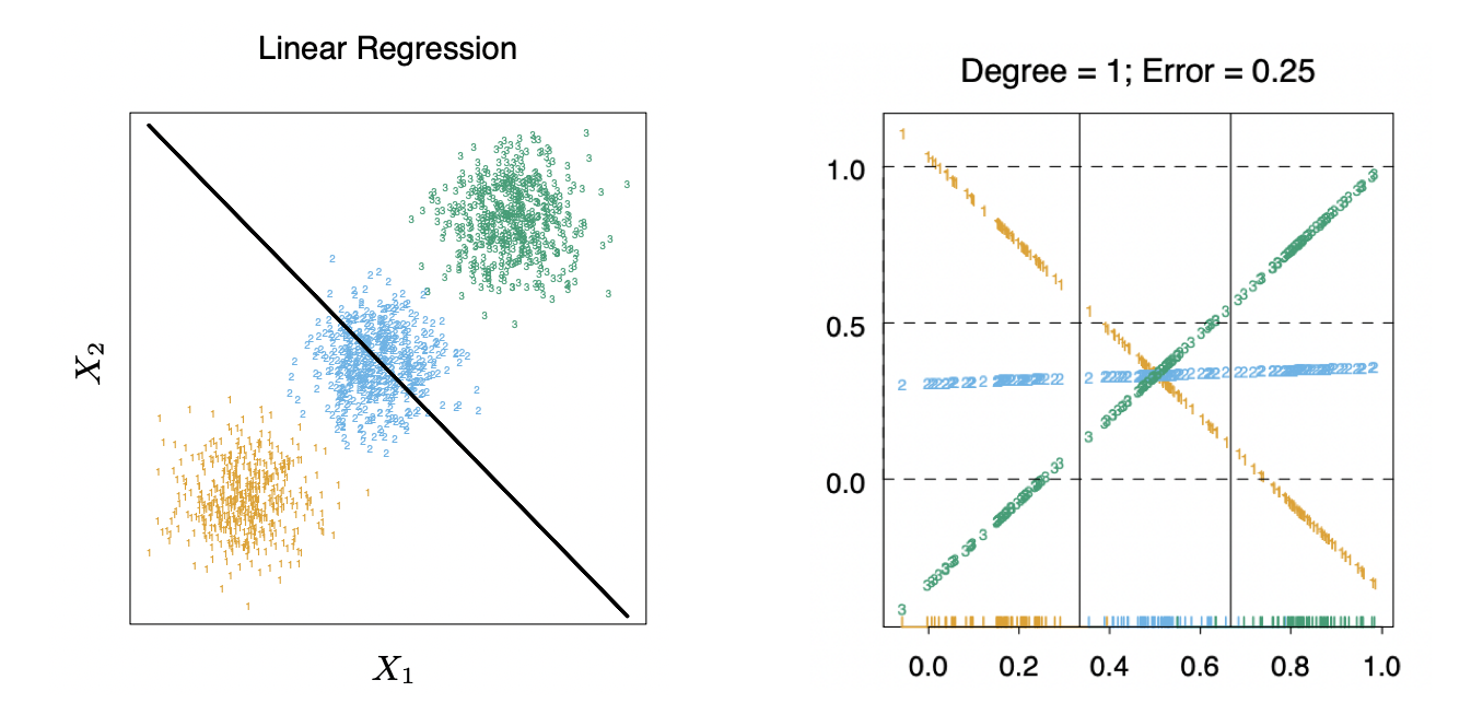
In this simple setting where the data in three different classes ligned up in a traight line, linear regression fail to discriminate class 2 (green) since the discriminant function of class 2 is never a maximum. (source: Elements of Statistical Learning)
It is known as a rule of thumb that to discriminate data in $K$ classes well, we need $(K-1)$ order of polynomial regression. This makes linear regression impractical, so LDA (QDA) and logistic regression is here to help.
LDA and QDA
We model the likelihood for LDA as
\[(X|Y=k) \sim \mathcal{N}(\mu_k, \Sigma)\]and for QDA as
\[(X|Y=k) \sim \mathcal{N}(\mu_k, \Sigma_k)\]for $k=1,\cdots,K.$ We construct the (linear) discriminant functions as before, and define a classifier as an argmax of them.
\[G(x) := \argmax_k \delta_k(x).\]Logistic regression
A in the binary case, we model the log odds as a linear function:
\[\log\frac{\mathbb{P}(Y=k|X=x)}{\mathbb{P}(Y\ne k|X=x)} \overset{\text{set}}{=} x^\intercal\boldsymbol{\beta}.\]Thus the resulting decision rule is
\[\mathbb{P}(Y=k|X=x) \propto e^{x^\intercal\boldsymbol\beta_k}, \\ \mathbb{P}(Y=k|X=x) = \frac{e^{x^\intercal\boldsymbol\beta_k}}{\sum_{l=1}^K e^{x^\intercal\boldsymbol\beta_l}},\]which is not idenfiable. We let $\boldsymbol\beta_1=\mathbf{0}$ for identifiability.
References
- Hastie, Tibshirani, Friedman. 2008. The Elements of Statistical Learning. 2nd edition. Springer.
- Advanced Data Mining (Spring, 2021) @ Seoul National University, Republic of Korea (instructor: Prof. Yongdai Kim).