Understanding Latent Dirichlet Allocation (3) Variational EM

Feb 15, 2021 • Sihyung Park
bayesian   machine learning   natural language processing  

$\newcommand{\argmin}{\mathop{\mathrm{argmin}}\limits}$ $\newcommand{\argmax}{\mathop{\mathrm{argmax}}\limits}$

Now that we know the structure of the model, it is time to fit the model parameters with real data. Among the possible inference methods, in this article I would like to explain the variational expectation-maximization algorithm.

This article is the third part of the series “Understanding Latent Dirichlet Allocation”.

1. Backgrounds
2. Model architecture
3. Inference - variational EM
4. Inference - Gibbs sampling
5. Smooth LDA

• Variational inference
• Variational EM
• Python implementation from scratch
  • E-step
  • M-step
  • Results

Variational inference

Variational inference (VI) is a method to approximate complicated distributions with a family of simpler surrogate distributions. In order to compute posterior distribution of latent variables given a document $\mathbf{w}_d$

\[p(\theta_d,\mathbf{z}_d|\mathbf{w_d},\alpha,\beta) = \frac{p(\theta_d, \mathbf{z}_d, \mathbf{w_d}|\alpha,\beta)}{p(\mathbf{w_d}|\alpha,\beta)},\]

it is necessary to compute the denominator

\[p(\mathbf{w_d}|\alpha,\beta) = \frac{\Gamma(\sum_i \alpha_i)}{\prod_i \Gamma(\alpha_i)} \int \left( \prod_{i=1}^k \theta_{di}^{\alpha_i-1} \right) \left( \prod_{n=1}^{N}\prod_{i=1}^k\prod_{j=1}^V (\theta_{di} \beta_{ij})^{w_{dn}^j} \right) d\theta.\]

However, it is intractable due to the coupling of $\theta$ and $\beta$ at the inner most parenthesis. Because of this, we utilize VI and Jensen’s inequality to achieve lower bound of the log likelihood $\log p(\mathbf{w}|\alpha,\beta)$ for parameter estimation of LDA.

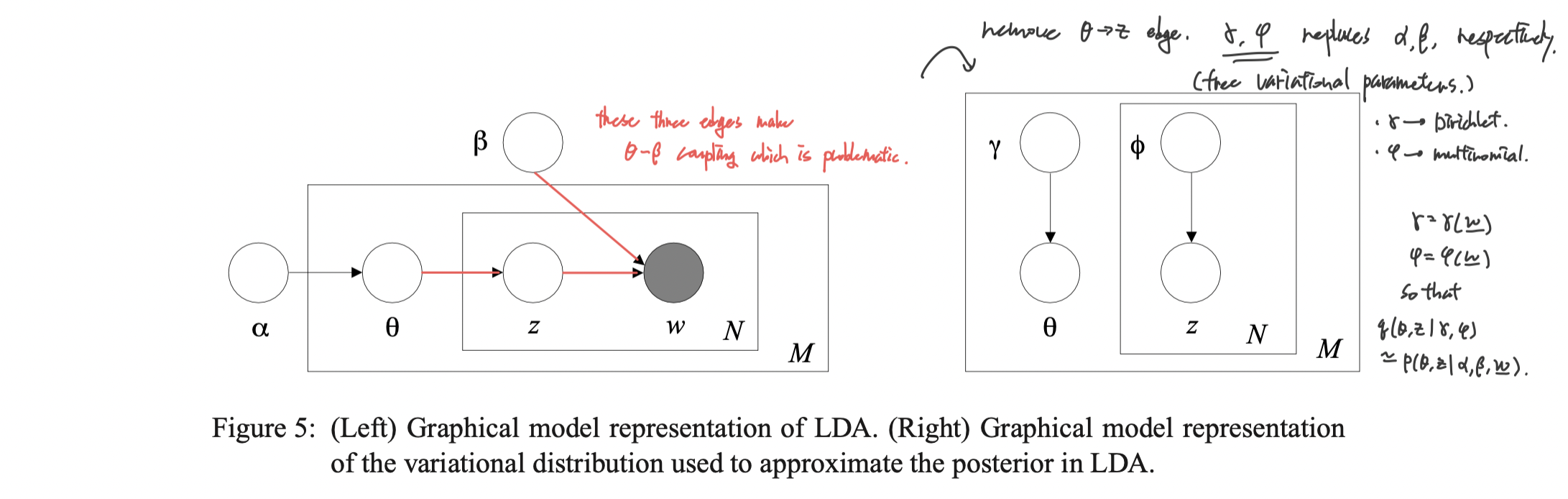
To be specific, we let the variational distribution $q$ to be parametrized by the variational parameters $\gamma=\gamma(\mathbf{w})$ and $\phi=\phi(\mathbf{w})$, each works similarly to $\alpha$ and $\beta$ of the true distribution, respectively. We set the variational distribution

\[q(\theta_d, \mathbf{z}_d|\gamma(\mathbf{w}_d),\phi(\mathbf{w}_d)) = q(\theta_d|\gamma(\mathbf{w}_d)) \prod_{n=1}^{N_d} q(z_{dn}|\phi_n(\mathbf{w}_d))\]

where

\[\theta_d \sim \mathcal{D}_k(\gamma(\mathbf{w}_d)), \\ z_{dn} \sim \mathcal{M}_k(\phi(\mathbf{w}_d)).\]

Graphical representation of the surrogate is depicted in the figure 5 of Blei et al. (2003).

Variational EM

Expectation maximization is a special case of minorization-maximization (MM) algorithm. I would like to use terminology from MM since it is more intuitive to explain the variational EM. To maximize a target likelihood function $f(x)$, EM algorithm works in the following way:

1. Set a family of simpler surrogate functions $\mathcal{G}$.
2. Repeat until convergence:
   1. (E-step) Minorize $f$ at $x^{(t)}$ with $g^{(t+1)}\in\mathcal{G}$.
   2. (M-step) Update $x^{(t+1)}=\arg\max g^{(t+1)}(x).$

Variational EM follows the framework of expectation-maximization, while uses variational inference to minorize the target function at the E-step. By Jensen’s inequality, we get the lower bound on the log likelihood with respect to the variational distribution defined above:

\[\begin{aligned} \log p(\mathbf{w}|\alpha,\beta) \ge \text{E}_q\log p(\theta,\mathbf{z},\mathbf{w}|\alpha,\beta) - \text{E}_q\log q(\theta,\mathbf{z}) =: L(\gamma,\phi|\alpha,\beta). \end{aligned}\]

Then variational EM algorithm for solving LDA is as follows:

1. Repeat until convergence:
   1. (E-step) Update $(\gamma^{(t+1)},\phi^{(t+1)}) = \arg\max_{(\gamma,\phi)} L(\gamma,\phi|\alpha^{(t)},\beta^{(t)})$.
   2. (M-step) Update $(\alpha^{(t+1)},\beta^{(t+1)}) = \arg\max_{(\alpha,\beta)} L(\gamma^{(t+1)},\phi^{(t+1)}|\alpha,\beta)$.

For $\beta$, $\phi$ and $\gamma$, closed form update formula can be easily derived by differentiating $L$, forming the Lagrangian and setting it to zero. I will leave this part for reading since it is a trivial, exhausting calculation well-described in appendix A.3 (Blei et al., 2003).

For $\alpha$, since $L$ has Hessian of the form $\text{diag}(h) + \mathbf{1}z\mathbf{1}’$, we use linear-time Newton-Raphson algorithm to update it.

To summarize, LDA solving variational EM algorithm repeats the following until the parameters converge.

• In the E-step, for $d=1,\cdots,M$,
  1. For $n=1,\cdots,N_d$ and $i=1,\cdots,k$,
     1. $\phi_{dni}^{(t+1)}=\beta_{iw_{dn}}\exp\left( \Psi(\gamma_{di}^{(t)}) - \Psi\big(\sum_{i=1}^k \gamma_{di}^{(t)}\big) \right)$.
  2. Normalize $\phi_{dn}^{(t+1)}$ to sum to $1$.
  3. $\gamma_d^{(t+1)}=\alpha^{(t)}+\sum_{n=1}^{N_d} \phi_{dn}^{(t+1)}$.
• In the M-step,
  1. $\beta_{ij}^{(t+1)} = \sum_{d=1}^M \sum_{n=1}^{N_d} \phi_{dni}^{(t+1)} \mathbf{w}_{dn}^j$.
  2. Update $\alpha^{(t+1)}$ with linear-time Newton method.

Here, $\Psi$ is the digamma function. I have yet clarified the update rule of linear-time Newton-Raphson algorithm. This is in appendix A.4.2 of Blei et al. (2003), which in its core is a mere block matrix inversion formula

\[(A+BCD)^{-1} = A^{-1} - A^{-1}B(C^{-1}+DA^{-1}B)^{-1}DA^{-1}.\]

So I will replace the explanation to Python implementation (_update()) below.

Python implementation from scratch

E-step

def E_step(docs, phi, gamma, alpha, beta):
    """
    Minorize the joint likelihood function via variational inference.
    This is the E-step of variational EM algorithm for LDA.
    """
    # optimize phi
    for m in range(M):
        phi[m, :N[m], :] = (beta[:, docs[m]] * np.exp(
            psi(gamma[m, :]) - psi(gamma[m, :].sum())
        ).reshape(-1, 1)).T

        # Normalize phi
        phi[m, :N[m]] /= phi[m, :N[m]].sum(axis=1).reshape(-1, 1)
        if np.any(np.isnan(phi)):
            raise ValueError("phi nan")

    # optimize gamma
    gamma = alpha + phi.sum(axis=1)

    return phi, gamma

It is the exact translation of the update equation at the above.

M-step

def M_step(docs, phi, gamma, alpha, beta, M):
    """
    maximize the lower bound of the likelihood.
    This is the M-step of variational EM algorithm for (smoothed) LDA.
    
    update of alpha follows from appendix A.2 of Blei et al., 2003.
    """
    # update alpha
    alpha = _update(alpha, gamma, M)
    
    # update beta
    for j in range(V):
        beta[:, j] = np.array(
            [_phi_dot_w(docs, phi, m, j) for m in range(M)]
        ).sum(axis=0)
    beta /= beta.sum(axis=1).reshape(-1, 1)

    return alpha, beta

This is also the exact replication of the equations, but with some abstraction for readability.

_update() is the implementation of linear-time Newton-Raphson algorithm.

import warnings

def _update(var, vi_var, const, max_iter=10000, tol=1e-6):
    """
    From appendix A.2 of Blei et al., 2003.
    For hessian with shape `H = diag(h) + 1z1'`
    
    To update alpha, input var=alpha and vi_var=gamma, const=M.
    To update eta, input var=eta and vi_var=lambda, const=k.
    """
    for _ in range(max_iter):
        # store old value
        var0 = var.copy()
        
        # g: gradient 
        psi_sum = psi(vi_var.sum(axis=1)).reshape(-1, 1)
        g = const * (psi(var.sum()) - psi(var)) \
            + (psi(vi_var) - psi_sum).sum(axis=0)

        # H = diag(h) + 1z1'
        ## z: Hessian constant component
        ## h: Hessian diagonal component
        z = const * polygamma(1, var.sum())
        h = -const * polygamma(1, var)
        c = (g / h).sum() / (1./z + (1./h).sum())

        # update var
        var -= (g - c) / h
        
        # check convergence
        err = np.sqrt(np.mean((var - var0) ** 2))
        crit = err < tol
        if crit:
            break
    else:
        warnings.warn(f"max_iter={max_iter} reached: values might not be optimal.")
    
    return var

_phi_dot_w() computes $\sum_{n=1}^{N_d} ϕ_{dni} w_{dn}^j$.

def _phi_dot_w(docs, phi, d, j):
    """
    \sum_{n=1}^{N_d} ϕ_{dni} w_{dn}^j
    """
    return (docs[d] == j) @ phi[d, :N[d], :]

Results

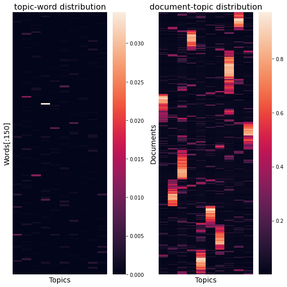
I ran LDA inference on $M=2000$ documents of Reuters News title data with $k=10$ topics. Top 9 important words in each topic (a mixture of word distribution) extracted from fitted LDA is as follows:

TOPIC 00: ['ec' 'csr' 'loss' 'bank' 'icco' 'unit' 'cocoa' 'fob' 'petroleum']
TOPIC 01: ['raises' 'acquisition' 'prices' 'prime' 'rate' 'w' 'completes' 'mar', 'imports']
TOPIC 02: ['year' 'sets' 'sees' 'net' 'stock' 'dividend' 'l' 'industries' 'corp']
TOPIC 03: ['pct' 'cts' 'gdp' 'opec' 'shr' 'february' 'plc' 'ups' 'rose']
TOPIC 04: ['u' 'japan' 'fed' 'trade' 'gaf' 'ems' 'says' 'dlr' 'gnp']
TOPIC 05: ['usda' 'f' 'ag' 'international' 'sell' 'report' 'ge' 'corn' 'wheat']
TOPIC 06: ['k' 'market' 'money' 'rate' 'eep' 'treasury' 'prime' 'says' 'mln']
TOPIC 07: ['qtr' 'note' '4th' 'net' 'loss' 'ico' 'corp' '1st' 'group']
TOPIC 08: ['dlrs' 'mln' 'bp' 'march' 'corp' 'week' 'canada' 'e' 'bank']
TOPIC 09: ['unit' 'buy' 'says' 'sale' 'c' 'sells' 'completes' 'american' 'grain']

Topic-word distribution ($\beta$) and document-topic distribution ($\theta$) recovered from LDA is as follows. $i$-th column from the figure left represents probabilities of each words to be generated given the topic $z_i$ so it sums to 1. Similarly, $d$-th row from the figure right represents the $d$-th document($\mathbf{w}_d$)’s mixture weights on topics, so it also sums to 1.

Full code and result are available here (GitHub).

References

• Blei, Ng, Jordan. 2003. Latent Dirichlet Allocation. Journal of Machine Learning Research. 3 (4–5): 993–1022.