Understanding Latent Dirichlet Allocation (5) Smooth LDA

Feb 17, 2021 • Sihyung Park
bayesian   machine learning   natural language processing  

$\newcommand{\argmin}{\mathop{\mathrm{argmin}}\limits}$ $\newcommand{\argmax}{\mathop{\mathrm{argmax}}\limits}$

From background to two inference processes, I covered all the important details of LDA so far. One thing left over is a difference between (basic) LDA and smooth LDA. Consider this last post as a cherry on top.

This article is the fifth and the final part of the series “Understanding Latent Dirichlet Allocation”.

1. Backgrounds
2. Model architecture
3. Inference - variational EM
4. Inference - Gibbs sampling
5. Smooth LDA

• Empirical vs. fuller Bayes
• Smooth LDA
• Variational EM for smooth LDA
  • E-step
  • M-step

Empirical vs. fuller Bayes

Not every Bayesian approches are the same. One of the most important aspect when applying Bayesian model to real-world data is decision of hyperparameters. For the task, empirical Bayes method “fit” the model to the data to derive, in many times, point estimate of hyperparameter, while standard (fuller) Bayes predefine the prior distribution before any data and update it later using the data as an evidence.

Recall the basic LDA that I explained from the first to the third articles. Pay attention to the part that hyperparameter $\beta$ does not have a distribution; it is assumed to be an unknown but fixed value. This makes the basic LDA an empirical Bayes model. Can we extend this to make a fuller Bayes model?

Smooth LDA

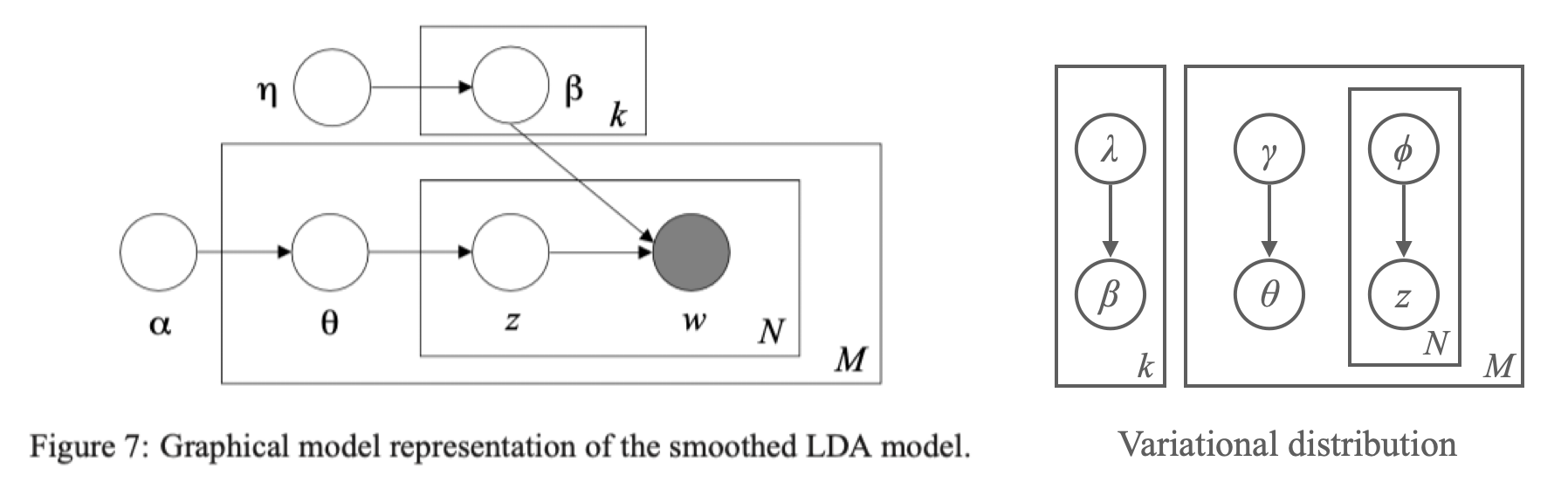
In order to extend the model to be fully Bayesian, all we need to do is to regard $\beta$ as another hidden parameter by endowing $\beta$ a Dirichlet prior $\beta_i \sim \mathcal{D}_V(\vec\eta)$ for all $i=1,\cdots,k$ where $\vec\eta=(\eta,\cdots,\eta)$ is a $V$-length vectors of the same elements $\eta $ by exchangeability. Blei et al. (2003) provides a graphical representation of this extended, or smoothed version of LDA. I added a modified variational distribution for it next to the figure.

So why would we want to make a model fully Bayesian? This is because of generability. If we use fixed point estimate for $\beta$, we get word-topic assignment that assigns probability zero to words that were not in training data. By giving $\beta$ a distribution, we can smooth it out to assign positive probability to all known and unknown words. In this perspective, fuller Bayes method can be seen as a smoothing method for hierarchical models.

Variational EM for smooth LDA

I already explained inference methods for smooth LDA: Gibbs sampling with Metropolis-Hastings rule proposed by Pritchard et al. (2000), and Collapsed gibbs sampling that Griffiths and Steyvers (2002) proposed are the ones. Here I would like to continue the discussion and be more specific on variational EM method that Blei et al. (2003) presented. If you are not familiar with variational EM algorithm, please take a look at the previous articles before moving on.

E-step

As in the figure that I put next to the Figure 7, we add additional variational parameter $\lambda$ that acts as a surrogate of $\eta$ and consider $\beta_i \sim \mathcal{D}_V(\lambda_i)$ for $i=1,\cdots,k$. Then the variational distribution becomes

\[q(\theta, \mathbf{z}, \beta|\gamma,\phi,\lambda) = \prod_{i=1}^k \mathcal{D}_V(\beta_i|\lambda_i) \prod_{d=1}^M q\big(\theta_d, \mathbf{z}_d|\gamma(\mathbf{w}_d),\phi(\mathbf{w}_d)\big)\]

Since $\beta$ part is multiplicative to the others, update rule for $\phi$ and $\gamma$ remains the same. (Actually, update rule of $\phi$ changes a little as it contains a $\beta$ term which is now considered a random variable.) Update rule for $\lambda$ is easy to derive by (again) differentiating the variational lower bound $L$ and setting it to zero.

There were no derivation depicted in the Blei et al. (2003), so I did one by myself. The variational lower bound $L$ is

\[\begin{aligned} L(\gamma,\phi,\lambda | \alpha,\eta) &= \sum_{i=1}^k \left( \log\Gamma(V\eta) - V\log\Gamma(\eta) + (\eta\cancel{-1}) \sum_{j=1}^V \bigg(\Psi(\lambda_{ij}) - \Psi\bigg(\sum_{j=1}^V\lambda_{ij}\bigg)\bigg) \right) \\ &+ \sum_{d=1}^M\left(\log\Gamma\biggr(\sum_{i=1}^k\alpha_i\biggr) - \sum_{i=1}^k \log\Gamma(\alpha_i) + \sum_{i=1}^k(\alpha_i-1)\left( \Psi(\gamma_{di}) - \Psi\biggr(\sum_{i=1}^k \gamma_{di}\biggr) \right)\right) \\ &+ \sum_{d=1}^M\sum_{n=1}^{N_d}\sum_{i=1}^k \phi_{dni}\left(\Psi(\gamma_{di}) - \Psi\biggr(\sum_{i=1}^k \gamma_{di}\biggr)\right) \\ &+ \sum_{d=1}^M\sum_{n=1}^{N_d}\sum_{i=1}^k\sum_{j=1}^V \phi_{dni}w_{dn}^j\left( \Psi(\lambda_{ij}) - \Psi\bigg(\sum_{j=1}^V\lambda_{ij}\bigg) \right) \\ &- \sum_{i=1}^k \left( \log\Gamma\bigg(\sum_{j=1}^V\lambda_{ij}\bigg) - \sum_{j=1}^V\log\Gamma(\lambda_{ij}) + \sum_{j=1}^V(\lambda_{ij}\cancel{-1})\bigg( \Psi(\lambda_{ij})-\Psi\bigg(\sum_{j=1}^V\lambda_{ij}\bigg) \bigg) \right) \\ &- \sum_{d=1}^M \left( \log\Gamma\biggr(\sum_{i=1}^k \gamma_{di}\biggr) - \sum_{i=1}^k \log\Gamma(\gamma_{di}) + \sum_{i=1}^k(\gamma_{di}-1)\biggr(\Psi(\gamma_{di}) - \Psi\biggr(\sum_{i=1}^k \gamma_{di}\biggr)\biggr) \right) \\ &- \sum_{d=1}^M\sum_{n=1}^{N_d}\sum_{i=1}^k \phi_{dni}\log\phi_{dni} . \end{aligned}\]

Organize only the terms with $\lambda_{ij}$ and differentiate it then we get

\[\begin{aligned} \frac{\partial L}{\partial \lambda_{ij}} = &~ \eta \color{blue}{ \left( \Psi'(\lambda_{ij}) - \Psi'\bigg(\sum_{j=1}^V\lambda_{ij}\bigg) \right) } \\ &+ \sum_{d=1}^M\sum_{n=1}^{N_d} \phi_{dni} w_{dn}^j \color{blue}{ \left( \Psi'(\lambda_{ij}) - \Psi'\bigg(\sum_{j=1}^V\lambda_{ij}\bigg) \right) } \\ &- \cancel{ M \left( \Psi\bigg(\sum_{j=1}^V \lambda_{ij}\bigg) - \Psi\left(\lambda_{ij}\right) \right) } \\ &- \cancel{ M \left( \Psi(\lambda_{ij}) - \Psi\bigg( \sum_{j=1}^V \lambda_{ij} \bigg) \right) } \\ &- \lambda_{ij} \color{blue}{ \left( \Psi'(\lambda_{ij}) - \Psi'\bigg(\sum_{j=1}^V \lambda_{ij}\bigg) \right) } \\ \end{aligned}\]

Thus letting it zero yields the update rule for $\lambda$:

\[\lambda_{ij}^{(t+1)} = \eta^{(t)} + \sum_{d=1}^M\sum_{n=1}^{N_d} \phi_{dni}^{(t)}w_{dn}^j.\]

M-step

Update rule for $\alpha$ is the same: we update it using linear-time Newton-Raphson. What is important is that update rule for $\eta$ is also the same as $\alpha$. It can be confirmed by organizing only the terms with $\eta$.

\[L_{[\eta]} = \sum_{i=1}^k \left( \log\Gamma(V \eta) - V\log\Gamma(\eta) + (\eta-1) \sum_{j=1}^V \bigg( \Psi(\lambda_{ij}) - \Psi\bigg(\sum_{j=1}^V\lambda_{ij}\bigg) \bigg) \right).\]

This is exactly the same as $L_{[\alpha]}$ if replacing $\eta$ with $\alpha$, $k$ with $M$, and $\eta$ with $\gamma$. (Recall that $\vec\eta$ is a vector of all the same elements) Thus by exactly the same algorithm (implemented as _update()), we can update $\eta$.

To summarize, the whole process of variational EM is as follows: First, initialize $\phi_{dni}^{(0)} := 1/k$ for all $i=1,\cdots,k$, $n=1,\cdots,N_d$ and $d=1,\cdots,M$ along with $\gamma_{di}^{(0)} := \alpha_i^{(0)} + N/k$ for all $i=1,\cdots,k$, $d=1,\cdots,M$. Then repeat the following until convergence.

1. In the E-step, for $d=1,\cdots,M$,
   1. For $n=1$ to $N$ and $i=1$ to $k$,
      1. $\phi_{dni}^{(t+1)} = \exp\left(\Psi(\lambda_{ij}^{(t)}) - \Psi\big(\sum_{j=1}^V \lambda_{ij}^{(t)}\big) + \Psi(\gamma_{di}^{(t)} - \Psi\big(\sum_{i=1}^k \gamma_{di}^{(t)}\big)\right)$.
      2. For $j=1, \cdots, V$,
         1. $\lambda_{ij}^{(t+1)} = \eta^{(t)} + \sum_{d=1}^M\sum_{n=1}^{N_d} \phi_{dni}^{(t+1)} w_{dn}^j$.
   2. Normalize $\phi_{dn}^{(t+1)}$ to sum to 1.
   3. $\gamma_d^{(t+1)} = \alpha + \sum_{n=1}^{N_d} \phi_{dni}^{(t+1)}$.
2. In the M-step,
   1. Update $\alpha^{(t+1)}$ with linear-time Newton-Raphson.
   2. Update $\vec\eta^{(t+1)}$ with linear-time Newton-Raphson.

Python code for the algorithm is in the last part of this notebook (GitHub).

References

• Blei, Ng, Jordan. 2003. Latent Dirichlet Allocation. Journal of Machine Learning Research. 3 (4–5): 993–1022.