Understanding Latent Dirichlet Allocation (2) The Model
In the last article, topic models frequently used at the time of development of LDA was covered. At the end of the post, I briefly introduced the rationale behind LDA. In this post, I would like to elaborate on details of the model architecture.
This article is the second part of the series “Understanding Latent Dirichlet Allocation”.
Generative process
Suppose we have a corpus with vocabulary of size $V$ and every words $w$ and every topics $z$ are one-hot encoded (i.e. $w^i=1$ and $w^j=0, j\ne i$ if $w$ is the i-th term in the vocabulary). Define a document $\mathbf{w}$ as a finite sequence of $N$ words
\[\mathbf{w} = (w_1, \cdots, w_N)\]and denote a corpus $D$ of $M$ documents
\[D = \{\mathbf{w}_1, \cdots, \mathbf{w}_M\}.\]For $k$ prespecified number of topics, LDA assumes that a $d$-th document $\mathbf{w}_d \in D$ with length $N_d$ is “generated” in the following steps1:
- $\theta_d \sim \mathcal{D}_k(\alpha)$. The multinomial parameter $\theta_d \in \mathbb{R}^k$ is drawn from $k$-dimensional Dirichlet distribution.
- For each words $w_{dn}, n=1,\cdots,N_d$ in the document:
- $z_{dn} \sim \mathcal{M}_k(1, \theta_d)$. A topic $z_{dn}$ for a word $w_{dn}$ is drawn from $k$-dim multinomial distribution.
- $w_{dn} | z_{dn}, \beta \sim \mathcal{M}_V(1, \beta_{i:z_{dn}^i=1})$. A word $w_{dn}$ given the topic $z_{dn}$ is drawn from $V$-dim multinomial distribution.
$\alpha \in \mathbb{R}^k, \beta \in \mathbb{R}^{k \times V}$ are hyperparameters that is common to all of the documents in a corpus. $\beta$ is an unknown constant that satisfies $\beta_{ij} = P(w^j=1|z^i=1)$. That is, given a topic $z$ such that $z^i = 1$, probability of $w_n$ given $\beta$ follows multinomial distribution with parameter $\beta_i$.
$\theta = (\theta_1, \cdots, \theta_M) \in \mathbb{R}^{M \times k}$ can be seen as the document-specific random topic matrix as $\theta_d$ generates topic for each words in $d$-th document as in the process.
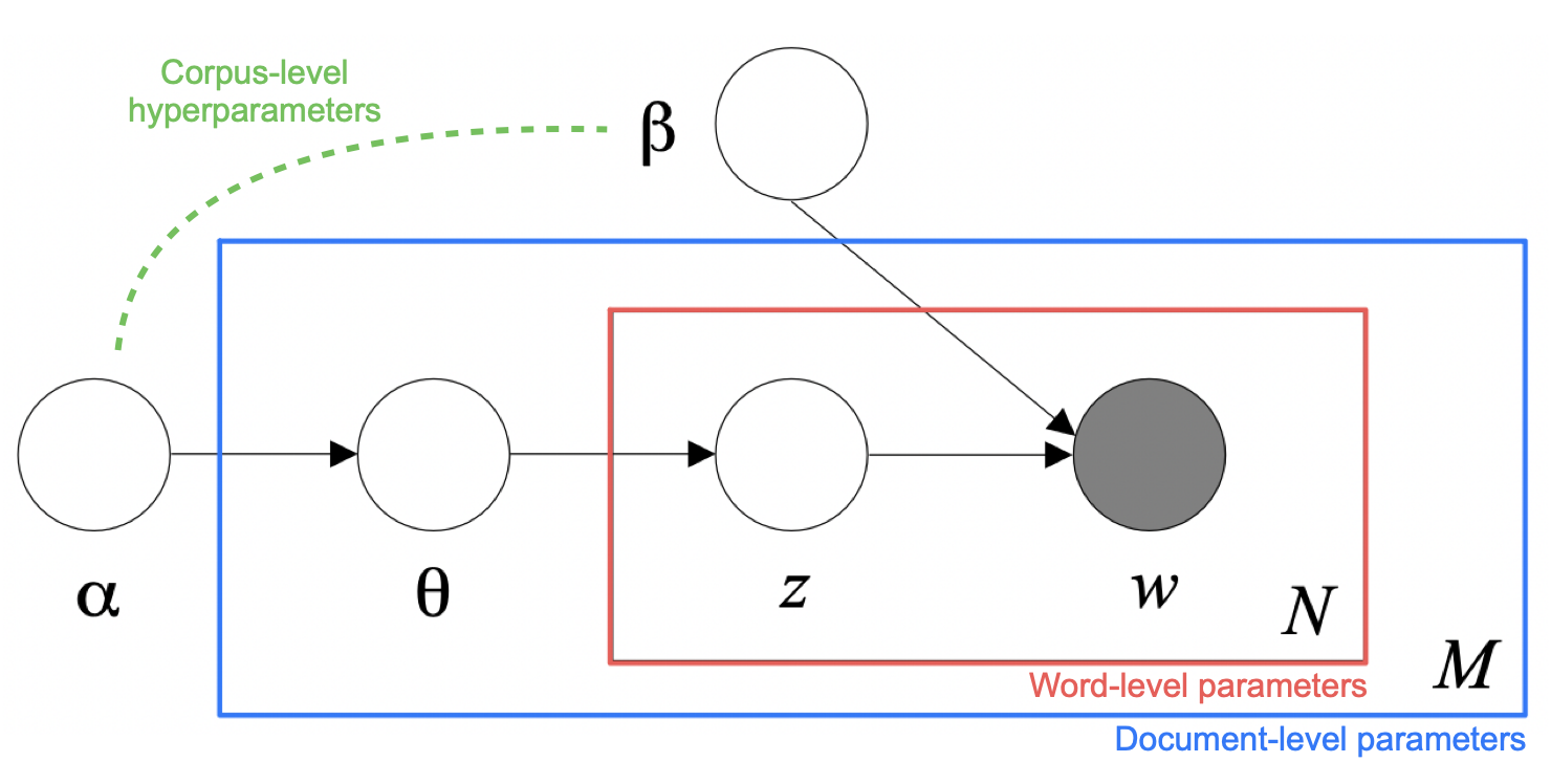
Blei et al. presented a graphical representation of the model. This helps understanding the structure as it illustrates the “scope” of each parameters. Only the words $w_{dn}$’s, that are filled with grey, are observable. Note that each word $w$ is generated by $z$ which is generated by $\theta$ which is again generated by $\alpha$; This makes LDA a three-level hierarchical model.
Mixture representations
In the previous article, I mentioned that under LDA model both words and documents can be represented as mixture distributions by de Finetti’s theorem. This property takes full advantage of bag-of-words assumption to reduce the number of parameters in large corpus and makes LDA a proper document model. Here, I would like to elaborate on it.
Words
By marginalizing over topics $z$, the word distribution is given by
\[P(w_{dn}|\theta_d, \beta) = \sum_z P(w_{dn}|z, \beta) P(z|\theta_d),\]where it is a mixture distribution of mixture weights $P(z|\theta_d)$ and components $P(w_{dn}|z,\beta)$.
Documents
We assumed in LDA that words are generated by topics and topics are exchangable within a document. Thus the joint density of $\theta_d, \mathbf{z}_d, \mathbf{w}_d$ is
\[p(\theta_d, \mathbf{z}_d, \mathbf{w}_d|\alpha, \beta) = P(\theta_d|\alpha)\prod_{n=1}^{N_d} P(z_{dn}|\theta_d)p(w_{dn}|z_{dn}, \beta)\]Marginalize it over $z$ and use the mixture representation of word distribution to get
\[p(\theta_d, \mathbf{w}_d | \alpha, \beta) = P(\theta_d|\alpha)\prod_{n=1}^{N_d} P(w_{dn}|\theta_d, \beta).\]Marginalize again with respect to $\theta_d$ and we get the continuous mixture representation of the document $\mathbf{w}_d$
\[p(\mathbf{w}_d | \alpha, \beta) = \int P(\theta_d|\alpha)\prod_{n=1}^{N_d} P(w_{dn}|\theta_d, \beta) ~d\theta_d,\]where $P(\theta_d|\alpha)$ are weights and $\prod_{n=1}^{N_d} P(w_{dn}|\theta_d, \beta)$ are components.
References
- Blei, Ng, Jordan. 2003. Latent Dirichlet Allocation. Journal of Machine Learning Research. 3 (4–5): 993–1022.
-
The number of words in a document is determined by Poisson distribution ($N \sim \mathcal{P}(\xi)$). I omitted this part because $N$ is an ancillary variable and it does not make the model description different even if it is considered as a constant. ↩